Automated Machine Learning (AutoML) refers to techniques for automatically discovering well-performing models for predictive modeling tasks with very little user involvement.
TPOT is an open-source library for performing AutoML in Python. It makes use of the popular Scikit-Learn machine learning library for data transforms and machine learning algorithms and uses a Genetic Programming stochastic global search procedure to efficiently discover a top-performing model pipeline for a given dataset.
In this tutorial, you will discover how to use TPOT for AutoML with Scikit-Learn machine learning algorithms in Python.
After completing this tutorial, you will know:
- TPOT is an open-source library for AutoML with scikit-learn data preparation and machine learning models.
- How to use TPOT to automatically discover top-performing models for classification tasks.
- How to use TPOT to automatically discover top-performing models for regression tasks.
Let’s get started.

TPOT for Automated Machine Learning in Python
Photo by Gwen, some rights reserved.
Tutorial Overview
This tutorial is divided into four parts; they are:
- TPOT for Automated Machine Learning
- Install and Use TPOT
- TPOT for Classification
- TPOT for Regression
TPOT for Automated Machine Learning
Tree-based Pipeline Optimization Tool, or TPOT for short, is a Python library for automated machine learning.
TPOT uses a tree-based structure to represent a model pipeline for a predictive modeling problem, including data preparation and modeling algorithms and model hyperparameters.
… an evolutionary algorithm called the Tree-based Pipeline Optimization Tool (TPOT) that automatically designs and optimizes machine learning pipelines.
— Evaluation of a Tree-based Pipeline Optimization Tool for Automating Data Science, 2016.
An optimization procedure is then performed to find a tree structure that performs best for a given dataset. Specifically, a genetic programming algorithm, designed to perform a stochastic global optimization on programs represented as trees.
TPOT uses a version of genetic programming to automatically design and optimize a series of data transformations and machine learning models that attempt to maximize the classification accuracy for a given supervised learning data set.
— Evaluation of a Tree-based Pipeline Optimization Tool for Automating Data Science, 2016.
The figure below taken from the TPOT paper shows the elements involved in the pipeline search, including data cleaning, feature selection, feature processing, feature construction, model selection, and hyperparameter optimization.
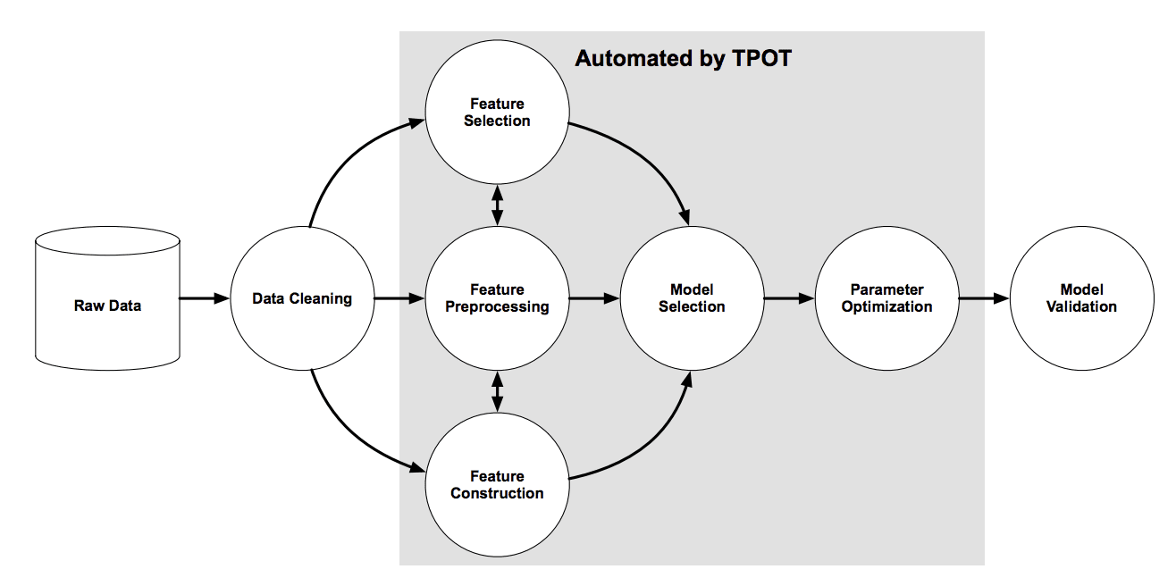
Overview of the TPOT Pipeline Search
Taken from: Evaluation of a Tree-based Pipeline Optimization Tool for Automating Data Science, 2016.
Now that we are familiar with what TPOT is, let’s look at how we can install and use TPOT to find an effective model pipeline.
Install and Use TPOT
The first step is to install the TPOT library, which can be achieved using pip, as follows:
pip install tpot
Once installed, we can import the library and print the version number to confirm it was installed successfully:
# check tpot version
import tpot
print('tpot: %s' % tpot.__version__)
Running the example prints the version number.
Your version number should be the same or higher.
tpot: 0.11.1
Using TPOT is straightforward.
It involves creating an instance of the TPOTRegressor or TPOTClassifier class, configuring it for the search, and then exporting the model pipeline that was found to achieve the best performance on your dataset.
Configuring the class involves two main elements.
The first is how models will be evaluated, e.g. the cross-validation scheme and performance metric. I recommend explicitly specifying a cross-validation class with your chosen configuration and the performance metric to use.
For example, RepeatedKFold for regression with ‘neg_mean_absolute_error‘ metric for regression:
...
# define evaluation procedure
cv = RepeatedKFold(n_splits=10, n_repeats=3, random_state=1)
# define search
model = TPOTRegressor(... scoring='neg_mean_absolute_error', cv=cv)
Or a RepeatedStratifiedKFold for regression with ‘accuracy‘ metric for classification:
...
# define evaluation procedure
cv = RepeatedStratifiedKFold(n_splits=10, n_repeats=3, random_state=1)
# define search
model = TPOTClassifier(... scoring='accuracy', cv=cv)
The other element is the nature of the stochastic global search procedure.
As an evolutionary algorithm, this involves setting configuration, such as the size of the population, the number of generations to run, and potentially crossover and mutation rates. The former importantly control the extent of the search; the latter can be left on default values if evolutionary search is new to you.
For example, a modest population size of 100 and 5 or 10 generations is a good starting point.
...
# define search
model = TPOTClassifier(generations=5, population_size=50, ...)
At the end of a search, a Pipeline is found that performs the best.
This Pipeline can be exported as code into a Python file that you can later copy-and-paste into your own project.
...
# export the best model
model.export('tpot_model.py')
Now that we are familiar with how to use TPOT, let’s look at some worked examples with real data.
TPOT for Classification
In this section, we will use TPOT to discover a model for the sonar dataset.
The sonar dataset is a standard machine learning dataset comprised of 208 rows of data with 60 numerical input variables and a target variable with two class values, e.g. binary classification.
Using a test harness of repeated stratified 10-fold cross-validation with three repeats, a naive model can achieve an accuracy of about 53 percent. A top-performing model can achieve accuracy on this same test harness of about 88 percent. This provides the bounds of expected performance on this dataset.
The dataset involves predicting whether sonar returns indicate a rock or simulated mine.
No need to download the dataset; we will download it automatically as part of our worked examples.
The example below downloads the dataset and summarizes its shape.
# summarize the sonar dataset
from pandas import read_csv
# load dataset
url = 'https://raw.githubusercontent.com/jbrownlee/Datasets/master/sonar.csv'
dataframe = read_csv(url, header=None)
# split into input and output elements
data = dataframe.values
X, y = data[:, :-1], data[:, -1]
print(X.shape, y.shape)
Running the example downloads the dataset and splits it into input and output elements. As expected, we can see that there are 208 rows of data with 60 input variables.
(208, 60) (208,)
Next, let’s use TPOT to find a good model for the sonar dataset.
First, we can define the method for evaluating models. We will use a good practice of repeated stratified k-fold cross-validation with three repeats and 10 folds.
...
# define model evaluation
cv = RepeatedStratifiedKFold(n_splits=10, n_repeats=3, random_state=1)
We will use a population size of 50 for five generations for the search and use all cores on the system by setting “n_jobs” to -1.
...
# define search
model = TPOTClassifier(generations=5, population_size=50, cv=cv, scoring='accuracy', verbosity=2, random_state=1, n_jobs=-1)
Finally, we can start the search and ensure that the best-performing model is saved at the end of the run.
...
# perform the search
model.fit(X, y)
# export the best model
model.export('tpot_sonar_best_model.py')
Tying this together, the complete example is listed below.
# example of tpot for the sonar classification dataset
from pandas import read_csv
from sklearn.preprocessing import LabelEncoder
from sklearn.model_selection import RepeatedStratifiedKFold
from tpot import TPOTClassifier
# load dataset
url = 'https://raw.githubusercontent.com/jbrownlee/Datasets/master/sonar.csv'
dataframe = read_csv(url, header=None)
# split into input and output elements
data = dataframe.values
X, y = data[:, :-1], data[:, -1]
# minimally prepare dataset
X = X.astype('float32')
y = LabelEncoder().fit_transform(y.astype('str'))
# define model evaluation
cv = RepeatedStratifiedKFold(n_splits=10, n_repeats=3, random_state=1)
# define search
model = TPOTClassifier(generations=5, population_size=50, cv=cv, scoring='accuracy', verbosity=2, random_state=1, n_jobs=-1)
# perform the search
model.fit(X, y)
# export the best model
model.export('tpot_sonar_best_model.py')
Running the example may take a few minutes, and you will see a progress bar on the command line.
Note: Your results may vary given the stochastic nature of the algorithm or evaluation procedure, or differences in numerical precision. Consider running the example a few times and compare the average outcome.
The accuracy of top-performing models will be reported along the way.
Generation 1 - Current best internal CV score: 0.8650793650793651
Generation 2 - Current best internal CV score: 0.8650793650793651
Generation 3 - Current best internal CV score: 0.8650793650793651
Generation 4 - Current best internal CV score: 0.8650793650793651
Generation 5 - Current best internal CV score: 0.8667460317460318

Best pipeline: GradientBoostingClassifier(GaussianNB(input_matrix), learning_rate=0.1, max_depth=7, max_features=0.7000000000000001, min_samples_leaf=15, min_samples_split=10, n_estimators=100, subsample=0.9000000000000001)
In this case, we can see that the top-performing pipeline achieved the mean accuracy of about 86.6 percent. This is a skillful model, and close to a top-performing model on this dataset.
The top-performing pipeline is then saved to a file named “tpot_sonar_best_model.py“.
Opening this file, you can see that there is some generic code for loading a dataset and fitting the pipeline. An example is listed below.
import numpy as np
import pandas as pd
from sklearn.ensemble import GradientBoostingClassifier
from sklearn.model_selection import train_test_split
from sklearn.naive_bayes import GaussianNB
from sklearn.pipeline import make_pipeline, make_union
from tpot.builtins import StackingEstimator
from tpot.export_utils import set_param_recursive

# NOTE: Make sure that the outcome column is labeled 'target' in the data file
tpot_data = pd.read_csv('PATH/TO/DATA/FILE', sep='COLUMN_SEPARATOR', dtype=np.float64)
features = tpot_data.drop('target', axis=1)
training_features, testing_features, training_target, testing_target = \
            train_test_split(features, tpot_data['target'], random_state=1)

# Average CV score on the training set was: 0.8667460317460318
exported_pipeline = make_pipeline(
    StackingEstimator(estimator=GaussianNB()),
    GradientBoostingClassifier(learning_rate=0.1, max_depth=7, max_features=0.7000000000000001, min_samples_leaf=15, min_samples_split=10, n_estimators=100, subsample=0.9000000000000001)
)
# Fix random state for all the steps in exported pipeline
set_param_recursive(exported_pipeline.steps, 'random_state', 1)

exported_pipeline.fit(training_features, training_target)
results = exported_pipeline.predict(testing_features)Note: as-is, this code does not execute, by design. It is a template that you can copy-and-paste into your project.
In this case, we can see that the best-performing model is a pipeline comprised of a Naive Bayes model and a Gradient Boosting model.
We can adapt this code to fit a final model on all available data and make a prediction for new data.
The complete example is listed below.
# example of fitting a final model and making a prediction on the sonar dataset
from pandas import read_csv
from sklearn.preprocessing import LabelEncoder
from sklearn.model_selection import RepeatedStratifiedKFold
from sklearn.ensemble import GradientBoostingClassifier
from sklearn.naive_bayes import GaussianNB
from sklearn.pipeline import make_pipeline
from tpot.builtins import StackingEstimator
from tpot.export_utils import set_param_recursive
# load dataset
url = 'https://raw.githubusercontent.com/jbrownlee/Datasets/master/sonar.csv'
dataframe = read_csv(url, header=None)
# split into input and output elements
data = dataframe.values
X, y = data[:, :-1], data[:, -1]
# minimally prepare dataset
X = X.astype('float32')
y = LabelEncoder().fit_transform(y.astype('str'))
# Average CV score on the training set was: 0.8667460317460318
exported_pipeline = make_pipeline(
    StackingEstimator(estimator=GaussianNB()),
    GradientBoostingClassifier(learning_rate=0.1, max_depth=7, max_features=0.7000000000000001, min_samples_leaf=15, min_samples_split=10, n_estimators=100, subsample=0.9000000000000001)
)
# Fix random state for all the steps in exported pipeline
set_param_recursive(exported_pipeline.steps, 'random_state', 1)
# fit the model
exported_pipeline.fit(X, y)
# make a prediction on a new row of data
row = [0.0200,0.0371,0.0428,0.0207,0.0954,0.0986,0.1539,0.1601,0.3109,0.2111,0.1609,0.1582,0.2238,0.0645,0.0660,0.2273,0.3100,0.2999,0.5078,0.4797,0.5783,0.5071,0.4328,0.5550,0.6711,0.6415,0.7104,0.8080,0.6791,0.3857,0.1307,0.2604,0.5121,0.7547,0.8537,0.8507,0.6692,0.6097,0.4943,0.2744,0.0510,0.2834,0.2825,0.4256,0.2641,0.1386,0.1051,0.1343,0.0383,0.0324,0.0232,0.0027,0.0065,0.0159,0.0072,0.0167,0.0180,0.0084,0.0090,0.0032]
yhat = exported_pipeline.predict([row])
print('Predicted: %.3f' % yhat[0])
Running the example fits the best-performing model on the dataset and makes a prediction for a single row of new data.
Predicted: 1.000
TPOT for Regression
In this section, we will use TPOT to discover a model for the auto insurance dataset.
The auto insurance dataset is a standard machine learning dataset comprised of 63 rows of data with one numerical input variable and a numerical target variable.
Using a test harness of repeated stratified 10-fold cross-validation with three repeats, a naive model can achieve a mean absolute error (MAE) of about 66. A top-performing model can achieve a MAE on this same test harness of about 28. This provides the bounds of expected performance on this dataset.
The dataset involves predicting the total amount in claims (thousands of Swedish Kronor) given the number of claims for different geographical regions.
- Auto Insurance Dataset (auto-insurance.csv)
- Auto Insurance Dataset Description (auto-insurance.names)
No need to download the dataset; we will download it automatically as part of our worked examples.
The example below downloads the dataset and summarizes its shape.
# summarize the auto insurance dataset
from pandas import read_csv
# load dataset
url = 'https://raw.githubusercontent.com/jbrownlee/Datasets/master/auto-insurance.csv'
dataframe = read_csv(url, header=None)
# split into input and output elements
data = dataframe.values
X, y = data[:, :-1], data[:, -1]
print(X.shape, y.shape)
Running the example downloads the dataset and splits it into input and output elements. As expected, we can see that there are 63 rows of data with one input variable.
(63, 1) (63,)
Next, we can use TPOT to find a good model for the auto insurance dataset.
First, we can define the method for evaluating models. We will use a good practice of repeated k-fold cross-validation with three repeats and 10 folds.
...
# define evaluation procedure
cv = RepeatedKFold(n_splits=10, n_repeats=3, random_state=1)
We will use a population size of 50 for 5 generations for the search and use all cores on the system by setting “n_jobs” to -1.
...
# define search
model = TPOTRegressor(generations=5, population_size=50, scoring='neg_mean_absolute_error', cv=cv, verbosity=2, random_state=1, n_jobs=-1)
Finally, we can start the search and ensure that the best-performing model is saved at the end of the run.
...
# perform the search
model.fit(X, y)
# export the best model
model.export('tpot_insurance_best_model.py')
Tying this together, the complete example is listed below.
# example of tpot for the insurance regression dataset
from pandas import read_csv
from sklearn.model_selection import RepeatedKFold
from tpot import TPOTRegressor
# load dataset
url = 'https://raw.githubusercontent.com/jbrownlee/Datasets/master/auto-insurance.csv'
dataframe = read_csv(url, header=None)
# split into input and output elements
data = dataframe.values
data = data.astype('float32')
X, y = data[:, :-1], data[:, -1]
# define evaluation procedure
cv = RepeatedKFold(n_splits=10, n_repeats=3, random_state=1)
# define search
model = TPOTRegressor(generations=5, population_size=50, scoring='neg_mean_absolute_error', cv=cv, verbosity=2, random_state=1, n_jobs=-1)
# perform the search
model.fit(X, y)
# export the best model
model.export('tpot_insurance_best_model.py')
Running the example may take a few minutes, and you will see a progress bar on the command line.
Note: Your results may vary given the stochastic nature of the algorithm or evaluation procedure, or differences in numerical precision. Consider running the example a few times and compare the average outcome.
The MAE of top-performing models will be reported along the way.
Generation 1 - Current best internal CV score: -29.147625969129034
Generation 2 - Current best internal CV score: -29.147625969129034
Generation 3 - Current best internal CV score: -29.147625969129034
Generation 4 - Current best internal CV score: -29.147625969129034
Generation 5 - Current best internal CV score: -29.147625969129034

Best pipeline: LinearSVR(input_matrix, C=1.0, dual=False, epsilon=0.0001, loss=squared_epsilon_insensitive, tol=0.001)
In this case, we can see that the top-performing pipeline achieved the mean MAE of about 29.14. This is a skillful model, and close to a top-performing model on this dataset.
The top-performing pipeline is then saved to a file named “tpot_insurance_best_model.py“.
Opening this file, you can see that there is some generic code for loading a dataset and fitting the pipeline. An example is listed below.
import numpy as np
import pandas as pd
from sklearn.model_selection import train_test_split
from sklearn.svm import LinearSVR

# NOTE: Make sure that the outcome column is labeled 'target' in the data file
tpot_data = pd.read_csv('PATH/TO/DATA/FILE', sep='COLUMN_SEPARATOR', dtype=np.float64)
features = tpot_data.drop('target', axis=1)
training_features, testing_features, training_target, testing_target = \
            train_test_split(features, tpot_data['target'], random_state=1)

# Average CV score on the training set was: -29.147625969129034
exported_pipeline = LinearSVR(C=1.0, dual=False, epsilon=0.0001, loss="squared_epsilon_insensitive", tol=0.001)
# Fix random state in exported estimator
if hasattr(exported_pipeline, 'random_state'):
    setattr(exported_pipeline, 'random_state', 1)

exported_pipeline.fit(training_features, training_target)
results = exported_pipeline.predict(testing_features)Note: as-is, this code does not execute, by design. It is a template that you can copy-paste into your project.
In this case, we can see that the best-performing model is a pipeline comprised of a linear support vector machine model.
We can adapt this code to fit a final model on all available data and make a prediction for new data.
The complete example is listed below.
# example of fitting a final model and making a prediction on the insurance dataset
from pandas import read_csv
from sklearn.model_selection import train_test_split
from sklearn.svm import LinearSVR
# load dataset
url = 'https://raw.githubusercontent.com/jbrownlee/Datasets/master/auto-insurance.csv'
dataframe = read_csv(url, header=None)
# split into input and output elements
data = dataframe.values
data = data.astype('float32')
X, y = data[:, :-1], data[:, -1]
# Average CV score on the training set was: -29.147625969129034
exported_pipeline = LinearSVR(C=1.0, dual=False, epsilon=0.0001, loss="squared_epsilon_insensitive", tol=0.001)
# Fix random state in exported estimator
if hasattr(exported_pipeline, 'random_state'):
    setattr(exported_pipeline, 'random_state', 1)
# fit the model
exported_pipeline.fit(X, y)
# make a prediction on a new row of data
row = [108]
yhat = exported_pipeline.predict([row])
print('Predicted: %.3f' % yhat[0])
Running the example fits the best-performing model on the dataset and makes a prediction for a single row of new data.
Predicted: 389.612
Further Reading
This section provides more resources on the topic if you are looking to go deeper.
- Evaluation of a Tree-based Pipeline Optimization Tool for Automating Data Science, 2016.
- TPOT Documentation.
- TPOT GitHub Project.
Summary
In this tutorial, you discovered how to use TPOT for AutoML with Scikit-Learn machine learning algorithms in Python.
Specifically, you learned:
- TPOT is an open-source library for AutoML with scikit-learn data preparation and machine learning models.
- How to use TPOT to automatically discover top-performing models for classification tasks.
- How to use TPOT to automatically discover top-performing models for regression tasks.
Do you have any questions?
Ask your questions in the comments below and I will do my best to answer.
The post TPOT for Automated Machine Learning in Python appeared first on Machine Learning Mastery.