MachineLearningMastery.com

What are the Benefits of Ensemble Methods for Machine Learning?

Ensembles are predictive models that combine predictions from two or more other models.

Ensemble learning methods are popular and the go-to technique when the best performance on a predictive modeling project is the most important outcome.

Nevertheless, they are not always the most appropriate technique to use and beginners the field of applied machine learning have the expectation that ensembles or a specific ensemble method are always the best method to use.

Ensembles offer two specific benefits on a predictive modeling project, and it is important to know what these benefits are and how to measure them to ensure that using an ensemble is the right decision on your project.

In this tutorial, you will discover the benefits of using ensemble methods for machine learning.

After reading this tutorial, you will know:

A minimum benefit of using ensembles is to reduce the spread in the average skill of a predictive model.
A key benefit of using ensembles is to improve the average prediction performance over any contributing member in the ensemble.
The mechanism for improved performance with ensembles is often the reduction in the variance component of prediction errors made by the contributing models.

Let’s get started.

Why Use Ensemble Learning
Photo by Juan Antonio Segal, some rights reseved.

Tutorial Overview

This tutorial is divided into four parts; they are:

Ensemble Learning
Use Ensembles to Improve Robustness
Bias, Variance, and Ensembles
Use Ensembles to Improve Performance

Ensemble Learning

An ensemble is a machine learning model that combines the predictions from two or more models.

The models that contribute to the ensemble, referred to as ensemble members, may be the same type or different types and may or may not be trained on the same training data.

The predictions made by the ensemble members may be combined using statistics, such as the mode or mean, or by more sophisticated methods that learn how much to trust each member and under what conditions.

The study of ensemble methods really picked up in the 1990s, and that decade was when papers on the most popular and widely used methods were published, such as core bagging, boosting, and stacking methods.

In the late 2000s, adoption of ensembles picked up due in part to their huge success in machine learning competitions, such as the Netflix prize and later competitions on Kaggle.

Over the last couple of decades, multiple classifier systems, also called ensemble systems have enjoyed growing attention within the computational intelligence and machine learning community.

— Page 1, Ensemble Machine Learning, 2012.

Ensemble methods greatly increase computational cost and complexity. This increase comes from the expertise and time required to train and maintain multiple models rather than a single model. This forces the question:

Why should we consider using an ensemble?

There are two main reasons to use an ensemble over a single model, and they are related; they are:

Performance: An ensemble can make better predictions and achieve better performance than any single contributing model.
Robustness: An ensemble reduces the spread or dispersion of the predictions and model performance.

Ensembles are used to achieve better predictive performance on a predictive modeling problem than a single predictive model. The way this is achieved can be understood as the model reducing the variance component of the prediction error by adding bias (i.e. in the context of the bias-variance trade-off).

Originally developed to reduce the variance—thereby improving the accuracy—of an automated decision-making system …

— Page 1, Ensemble Machine Learning, 2012.

There is another important and less discussed benefit of ensemble methods is improved robustness or reliability in the average performance of a model.

These are both important concerns on a machine learning project and sometimes we may prefer one or both properties from a model.

Let’s take a closer look at these two properties in order to better understand the benefits of using ensemble learning on a project.

Use Ensembles to Improve Robustness

On a predictive modeling project, we often evaluate multiple models or modeling pipelines and choose one that performs well or best as our final model.

The algorithm or pipeline is then fit on all available data and used to make predictions on new data.

We have an idea of how well the model will perform on average from our test harness, typically estimated using repeated k-fold cross-validation as a gold standard. The problem is, average performance might not be sufficient.

An average accuracy or error of a model is a summary of the expected performance, when in fact, some models performed better and some models performed worse on different subsets of the data.

The standard deviation is the average difference between an observation and the mean and summarizes the dispersion or spread of data. For an accuracy or error measure for a model, it can give you an idea of the spread of the model’s behavior.

Looking at the minimum and maximum model performance scores will give you an idea of the worst and best performance you might expect from the model, and this might not be acceptable for your application.

The simplest ensemble is to fit the model multiple times on the training datasets and combine the predictions using a summary statistic, such as the mean for regression or the mode for classification. Importantly, each model needs to be slightly different due to the stochastic learning algorithm, difference in the composition of the training dataset, or differences in the model itself.

This will reduce the spread in the predictions made by the model. The mean performance will probably be about the same, although the worst- and best-case performance will be brought closer to the mean performance.

In effect, it smooths out the expected performance of the model.

We can refer to this as the “robustness” in the expected performance of the model and is a minimum benefit of using an ensemble method.

An ensemble may or may not improve modeling performance over any single contributing member, discussed more further, but at minimum, it should reduce the spread in the average performance of the model.

For more on this topic, see the tutorial:

How to Reduce Variance in a Final Machine Learning Model

Bias, Variance, and Ensembles

Machine learning models for classification and regression learn a mapping function from inputs to outputs.

This mapping is learned from examples from the problem domain, the training dataset, and is evaluated on data not used during training, the test dataset.

The errors made by a machine learning model are often described in terms of two properties: the bias and the variance.

The bias is a measure of how close the model can capture the mapping function between inputs and outputs. It captures the rigidity of the model: the strength of the assumption the model has about the functional form of the mapping between inputs and outputs.

The variance of the model is the amount the performance of the model changes when it is fit on different training data. It captures the impact of the specifics of the data has on the model.

Variance refers to the amount by which [the model] would change if we estimated it using a different training data set.

— Page 34, An Introduction to Statistical Learning with Applications in R, 2014.

The bias and the variance of a model’s performance are connected.

Ideally, we would prefer a model with low bias and low variance, although in practice, this is very challenging. In fact, this could be described as the goal of applied machine learning for a given predictive modeling problem.

Reducing the bias can often easily be achieved by increasing the variance. Conversely, reducing the variance can easily be achieved by increasing the bias.

This is referred to as a trade-off because it is easy to obtain a method with extremely low bias but high variance […] or a method with very low variance but high bias …

— Page 36, An Introduction to Statistical Learning with Applications in R, 2014.

Some models naturally have a high bias or a high variance, which can be often relaxed or increased using hyperparameters that change the learning behavior of the algorithm.

Ensembles provide a way to reduce the variance of the predictions; that is the amount of error in the predictions made that can be attributed to “variance.”

This is not always the case, but when it is, this reduction in variance, in turn, leads to improved predictive performance.

Empirical and theoretical evidence show that some ensemble techniques (such as bagging) act as a variance reduction mechanism, i.e., they reduce the variance component of the error. Moreover, empirical results suggest that other ensemble techniques (such as AdaBoost) reduce both the bias and the variance parts of the error.

— Page 39, Pattern Classification Using Ensemble Methods, 2010.

Using ensembles to reduce the variance properties of prediction errors leads to the key benefit of using ensembles in the first place: to improve predictive performance.

Use Ensembles to Improve Performance

Reducing the variance element of the prediction error improves predictive performance.

We explicitly use ensemble learning to seek better predictive performance, such as lower error on regression or high accuracy for classification.

… there is a way to improve model accuracy that is easier and more powerful than judicious algorithm selection: one can gather models into ensembles.

— Page 2, Ensemble Methods in Data Mining, 2010.

This is the primary use of ensemble learning methods and the benefit demonstrated through the use of ensembles by the majority of winners of machine learning competitions, such as the Netflix prize and competitions on Kaggle.

In the Netflix Prize, a contest ran for two years in which the first team to submit a model improving on Netflix’s internal recommendation system by 10% would win $1,000,000. […] the final edge was obtained by weighing contributions from the models of up to 30 competitors.

— Page 8, Ensemble Methods in Data Mining, 2010.

This benefit has also been demonstrated with academic competitions, such as top solutions for the famous ImageNet dataset in computer vision.

An ensemble of these residual nets achieves 3.57% error on the ImageNet test set. This result won the 1st place on the ILSVRC 2015 classification task.

— Deep Residual Learning for Image Recognition, 2015.

When used in this way, an ensemble should only be adopted if it performs better on average than any contributing member of the ensemble. If this is not the case, then the contributing member that performs better should be used instead.

Consider the distribution of expected scores calculated by a model on a test harness, such as repeated k-fold cross-validation, as we did above when considering the “robustness” offered by an ensemble. An ensemble that reduces the variance in the error, in effect, will shift the distribution rather than simply shrink the spread of the distribution.

This can result in a better average performance as compared to any single model.

This is not always the case, and having this expectation is a common mistake made by beginners.

It is possible, and even common, for the performance of an ensemble to perform no better than the best-performing member of the ensemble. This can happen if the ensemble has one top-performing model and the other members do not offer any benefit or the ensemble is not able to harness their contribution effectively.

It is also possible for an ensemble to perform worse than the best-performing member of the ensemble. This too is common any typically involves one top-performing model whose predictions are made worse by one or more poor-performing other models and the ensemble is not able to harness their contributions effectively.

As such, it is important to test a suite of ensemble methods and tune their behavior, just as we do for any individual machine learning model.

Summary

In this post, you discovered the benefits of using ensemble methods for machine learning.

Specifically, you learned:

A minimum benefit of using ensembles is to reduce the spread in the average skill of a predictive model.
A key benefit of using ensembles is to improve the average prediction performance over any contributing member in the ensemble.
The mechanism for improved performance with ensembles is often the reduction in the variance component of prediction errors made by the contributing models.

Do you have any questions?
Ask your questions in the comments below and I will do my best to answer.

The post Why Use Ensemble Learning? appeared first on Machine Learning Mastery.

Machine learning algorithms, like logistic regression and support vector machines, are designed for two-class (binary) classification problems.

As such, these algorithms must either be modified for multi-class (more than two) classification problems or not used at all. The Error-Correcting Output Codes method is a technique that allows a multi-class classification problem to be reframed as multiple binary classification problems, allowing the use of native binary classification models to be used directly.

Unlike one-vs-rest and one-vs-one methods that offer a similar solution by dividing a multi-class classification problem into a fixed number of binary classification problems, the error-correcting output codes technique allows each class to be encoded as an arbitrary number of binary classification problems. When an overdetermined representation is used, it allows the extra models to act as “error-correction” predictions that can result in better predictive performance.

In this tutorial, you will discover how to use error-correcting output codes for classification.

After completing this tutorial, you will know:

Error-correcting output codes is a technique for using binary classification models on multi-class classification prediction tasks.
How to fit, evaluate, and use error-correcting output codes classification models to make predictions.
How to tune and evaluate different values for the number of bits per class hyperparameter used by error-correcting output codes.

Let’s get started.

Error-Correcting Output Codes (ECOC) for Machine Learning
Photo by Fred Hsu, some rights reserved.

Tutorial Overview

This tutorial is divided into three parts; they are:

Error-Correcting Output Codes
Evaluate and Use ECOC Classifiers
Tune Number of Bits Per Class

Error-Correcting Output Codes

Classification tasks are those where a label is predictive for a given input variable.

Binary classification tasks are those classification problems where the target contains two values, whereas multi-class classification problems are those that have more than two target class labels.

Many machine learning models have been developed for binary classification, although they may require modification to work with multi-class classification problems. For example, logistic regression and support vector machines were specifically designed for binary classification.

Several machine learning algorithms, such as SVM, were originally designed to solve only binary classification tasks.

— Page 133, Pattern Classification Using Ensemble Methods, 2010.

Rather than limiting the choice of algorithms or adapting the algorithms for multi-class problems, an alternative approach is to reframe the multi-class classification problem as multiple binary classification problems. Two common methods that can be used to achieve this include the one-vs-rest (OvR) and one-vs-one (OvO) techniques.

OvR: splits a multi-class problem into one binary problem per class.
OvO: splits a multi-class problem into one binary problem per each pair of classes.

Once split into subtasks, a binary classification model can be fit on each task and the model with the largest response can be taken as the prediction.

Both the OvR and OvO may be thought of as a type of ensemble learning model given that multiple separate models are fit for a predictive modeling task and used in concert to make a prediction. In both cases, the prediction of the “ensemble members” is a simple winner take all approach.

… convert the multiclass task into an ensemble of binary classification tasks, whose results are then combined.

— Page 134, Pattern Classification Using Ensemble Methods, 2010.

For more on one-vs-rest and one-vs-one models, see the tutorial:

How to Use One-vs-Rest and One-vs-One for Multi-Class Classification

A related approach is to prepare a binary encoding (e.g. a bitstring) to represent each class in the problem. Each bit in the string can be predicted by a separate binary classification problem. Arbitrarily, length encodings can be chosen for a given multi-class classification problem.

To be clear, each model receives the full input pattern and only predicts one position in the output string. During training, each model can be trained to produce the correct 0 or 1 output for the binary classification task. A prediction can then be made for new examples by using each model to make a prediction for the input to create the binary string, then compare the binary string to each class’s known encoding. The class encoding that has the smallest distance to the prediction is then chosen as the output.

A codeword of length l is ascribed to each class. Commonly, the size of the codewords has more bits than needed in order to uniquely represent each class.

— Page 138, Pattern Classification Using Ensemble Methods, 2010.

It is an interesting approach that allows the class representation to be more elaborate than is required (perhaps overdetermined) as compared to a one-hot encoding and introduces redundancy into the representation and modeling of the problem. This is intentional as the additional bits in the representation act like error-correcting codes to fix, correct, or improve the prediction.

… the idea is that the redundant “error-correcting” bits allow for some inaccuracies, and can improve performance.

— Page 606, The Elements of Statistical Learning, 2016.

This gives the technique its name: error-correcting output codes, or ECOC for short.

Error-Correcting Output Codes (ECOC) is a simple yet powerful approach to deal with a multi-class problem based on the combination of binary classifiers.

— Page 90, Ensemble Methods, 2012.

Care can be taken to ensure that each encoded class has a very different binary string encoding. A suite of different encoding schemes has been explored as well as specific methods for constructing the encodings to ensure they are sufficiently far apart in the encoding space. Interestingly, random encodings have been found to work perhaps just as well.

… analyzed the ECOC approach, and showed that random code assignment worked as well as the optimally constructed error-correcting codes

— Page 606, The Elements of Statistical Learning, 2016.

For a detailed review of the various different encoding schemes and methods for mapping predicted strings to encoded classes, I recommend Chapter 6 “Error Correcting Output Codes” of the book “Pattern Classification Using Ensemble Methods“.

Evaluate and Use ECOC Classifiers

The scikit-learn library provides an implementation of ECOC via the OutputCodeClassifier class.

The class takes as an argument the model to use to fit each binary classifier, and any machine learning model can be used. In this case, we will use a logistic regression model, intended for binary classification.

The class also provides the “code_size” argument that specifies the size of the encoding for the classes as a multiple of the number of classes, e.g. the number of bits to encode for each class label.

For example, if we wanted an encoding with bit strings with a length of 6 bits, and we had three classes, then we can specify the coding size as 2:

encoding_length = code_size * num_classes
encoding_length = 2 * 3
encoding_length = 6

The example below demonstrates how to define an example of the OutputCodeClassifier with 2 bits per class and using a LogisticRegression model for each bit in the encoding.

...
# define the binary classification model
model = LogisticRegression()
# define the ecoc model
ecoc = OutputCodeClassifier(model, code_size=2, random_state=1)

Although there are many sophisticated ways to construct the encoding for each class, the OutputCodeClassifier class selects a random bit string encoding for each class, at least at the time of writing.

We can explore the use of the OutputCodeClassifier on a synthetic multi-class classification problem.

We can use the make_classification() function to define a multi-class classification problem with 1,000 examples, 20 input features, and three classes.

The example below demonstrates how to create the dataset and summarize the number of rows, columns, and classes in the dataset.

# multi-class classification dataset
from collections import Counter
from sklearn.datasets import make_classification
# define dataset
X, y = make_classification(n_samples=1000, n_features=20, n_informative=15, n_redundant=5, random_state=1, n_classes=3)
# summarize the dataset
print(X.shape, y.shape)
# summarize the number of classes
print(Counter(y))

Running the example creates the dataset and reports the number of rows and columns, confirming the dataset was created as expected.

The number of examples in each class is then reported, showing a nearly equal number of cases for each of the three configured classes.

(1000, 20) (1000,)
Counter({2: 335, 1: 333, 0: 332})

Next, we can evaluate an error-correcting output codes model on the dataset.

We will use a logistic regression with 2 bits per class as we defined above. The model will then be evaluated using repeated stratified k-fold cross-validation with three repeats and 10 folds. We will summarize the performance of the model using the mean and and standard deviation of classification accuracy across all repeats and folds.

...
# define the evaluation procedure
cv = RepeatedStratifiedKFold(n_splits=10, n_repeats=3, random_state=1)
# evaluate the model and collect the scores
n_scores = cross_val_score(ecoc, X, y, scoring='accuracy', cv=cv, n_jobs=-1)
# summarize the performance
print('Accuracy: %.3f (%.3f)' % (mean(n_scores), std(n_scores)))

Tying this together, the complete example is listed below.

# evaluate error-correcting output codes for multi-class classification
from numpy import mean
from numpy import std
from sklearn.datasets import make_classification
from sklearn.model_selection import cross_val_score
from sklearn.model_selection import RepeatedStratifiedKFold
from sklearn.linear_model import LogisticRegression
from sklearn.multiclass import OutputCodeClassifier
# define dataset
X, y = make_classification(n_samples=1000, n_features=20, n_informative=15, n_redundant=5, random_state=1, n_classes=3)
# define the binary classification model
model = LogisticRegression()
# define the ecoc model
ecoc = OutputCodeClassifier(model, code_size=2, random_state=1)
# define the evaluation procedure
cv = RepeatedStratifiedKFold(n_splits=10, n_repeats=3, random_state=1)
# evaluate the model and collect the scores
n_scores = cross_val_score(ecoc, X, y, scoring='accuracy', cv=cv, n_jobs=-1)
# summarize the performance
print('Accuracy: %.3f (%.3f)' % (mean(n_scores), std(n_scores)))

Running the example defines the model and evaluates it on our synthetic multi-class classification dataset using the defined test procedure.

Note: Your results may vary given the stochastic nature of the algorithm or evaluation procedure, or differences in numerical precision. Consider running the example a few times and compare the average outcome.

In this case, we can see that the model achieved a mean classification accuracy of about 76.6 percent.

Accuracy: 0.766 (0.037)

We may choose to use this as our final model.

This requires that we fit the model on all available data and use it to make predictions on new data.

The example below provides a full example of how to fit and use an error-correcting output model as a final model.

# use error-correcting output codes model as a final model and make a prediction
from sklearn.datasets import make_classification
from sklearn.linear_model import LogisticRegression
from sklearn.multiclass import OutputCodeClassifier
# define dataset
X, y = make_classification(n_samples=1000, n_features=20, n_informative=15, n_redundant=5, random_state=1, n_classes=3)
# define the binary classification model
model = LogisticRegression()
# define the ecoc model
ecoc = OutputCodeClassifier(model, code_size=2, random_state=1)
# fit the model on the whole dataset
ecoc.fit(X, y)
# make a single prediction
row = [[0.04339387, 2.75542632, -3.79522705, -0.71310994, -3.08888853, -1.2963487, -1.92065166, -3.15609907, 1.37532356, 3.61293237, 1.00353523, -3.77126962, 2.26638828, -10.22368666, -0.35137382, 1.84443763, 3.7040748, 2.50964286, 2.18839505, -2.31211692]]
yhat = ecoc.predict(row)
print('Predicted Class: %d' % yhat[0])

Running the example fits the ECOC model on the entire dataset and uses the model to predict the class label for a single row of data.

In this case, we can see that the model predicted the class label 0.

Predicted Class: 0

Now that we are familiar with how to fit and use the ECOC model, let’s take a closer look at how to configure it.

Tune Number of Bits Per Class

The key hyperparameter for the ECOC model is the encoding of class labels.

This includes properties such as:

The choice of representation (bits, real numbers, etc.)
The encoding of each class label (random, etc.)
The length of representation (number of bits, etc.)
How predictions are mapped to classes (distance, etc.)

The OutputCodeClassifier scikit-learn implementation does not currently provide a lot of control over these elements.

The element it does give control over is the number of bits used to encode each class label.

In this section, we can perform a manual grid search across different numbers of bits per class label and compare the results. This provides a template that you can adapt and use on your own project.

First, we can define a function to create and return the dataset.

# get the dataset
def get_dataset():
	X, y = make_classification(n_samples=1000, n_features=20, n_informative=15, n_redundant=5, random_state=1, n_classes=3)
	return X, y

We can then define a function that will create a collection of models to evaluate.

Each model will be an example of the OutputCodeClassifier using a LogisticRegression for each binary classification problem. We will configure the code_size of each model to be different, with values ranging from 1 to 20.

# get a list of models to evaluate
def get_models():
	models = dict()
	for i in range(1,21):
		# create model
		model = LogisticRegression()
		# create error correcting output code classifier
		models[str(i)] = OutputCodeClassifier(model, code_size=i, random_state=1)
	return models

We can evaluate each model using related k-fold cross-validation as we did in the previous section to give a sample of classification accuracy scores.

# evaluate a give model using cross-validation
def evaluate_model(model):
	cv = RepeatedStratifiedKFold(n_splits=10, n_repeats=3, random_state=1)
	scores = cross_val_score(model, X, y, scoring='accuracy', cv=cv, n_jobs=-1)
	return scores

We can report the mean and standard deviation of the scores for each configuration and plot the distributions as box and whisker plots side by side to visually compare the results.

...
# evaluate the models and store results
results, names = list(), list()
for name, model in models.items():
	scores = evaluate_model(model)
	results.append(scores)
	names.append(name)
	print('>%s %.3f (%.3f)' % (name, mean(scores), std(scores)))
# plot model performance for comparison
pyplot.boxplot(results, labels=names, showmeans=True)
pyplot.show()

Tying this all together, the complete example of comparing ECOC classification with a grid of the number of bits per class is listed below.

# compare the number of bits per class for error-correcting output code classification
from numpy import mean
from numpy import std
from sklearn.datasets import make_classification
from sklearn.model_selection import cross_val_score
from sklearn.model_selection import RepeatedStratifiedKFold
from sklearn.linear_model import LogisticRegression
from sklearn.multiclass import OutputCodeClassifier
from matplotlib import pyplot

# get the dataset
def get_dataset():
	X, y = make_classification(n_samples=1000, n_features=20, n_informative=15, n_redundant=5, random_state=1, n_classes=3)
	return X, y

# get a list of models to evaluate
def get_models():
	models = dict()
	for i in range(1,21):
		# create model
		model = LogisticRegression()
		# create error correcting output code classifier
		models[str(i)] = OutputCodeClassifier(model, code_size=i, random_state=1)
	return models

# evaluate a give model using cross-validation
def evaluate_model(model):
	cv = RepeatedStratifiedKFold(n_splits=10, n_repeats=3, random_state=1)
	scores = cross_val_score(model, X, y, scoring='accuracy', cv=cv, n_jobs=-1)
	return scores

# define dataset
X, y = get_dataset()
# get the models to evaluate
models = get_models()
# evaluate the models and store results
results, names = list(), list()
for name, model in models.items():
	scores = evaluate_model(model)
	results.append(scores)
	names.append(name)
	print('>%s %.3f (%.3f)' % (name, mean(scores), std(scores)))
# plot model performance for comparison
pyplot.boxplot(results, labels=names, showmeans=True)
pyplot.show()

Running the example first evaluates each model configuration and reports the mean and standard deviation of the accuracy scores.

In this case, we can see that perhaps 5 or 6 bits per class results in the best performance with reported mean accuracy scores of about 78.2 percent and 78.0 percent respectively. We also see good results for 9, 13, 17, and 20 bits per class, with perhaps 17 bits per class giving the best result of about 78.5 percent.

>1 0.545 (0.032)
>2 0.766 (0.037)
>3 0.776 (0.036)
>4 0.769 (0.035)
>5 0.782 (0.037)
>6 0.780 (0.037)
>7 0.776 (0.039)
>8 0.775 (0.036)
>9 0.782 (0.038)
>10 0.779 (0.036)
>11 0.770 (0.033)
>12 0.777 (0.037)
>13 0.781 (0.037)
>14 0.779 (0.039)
>15 0.771 (0.033)
>16 0.769 (0.035)
>17 0.785 (0.034)
>18 0.776 (0.038)
>19 0.776 (0.034)
>20 0.780 (0.038)

A figure is created showing the box and whisker plots for the accuracy scores for each model configuration.

We can see that besides a value of 1, the number of bits per class delivers similar results in terms of spread and mean accuracy scores that cluster around 77 percent. This suggests that the approach is reasonably stable across configurations.

Box and Whisker Plots of Bits Per Class vs. Distribution of Classification Accuracy for ECOC

Summary

In this tutorial, you discovered how to use error-correcting output codes for classification.

Specifically, you learned:

Error-correcting output codes is a technique for using binary classification models on multi-class classification prediction tasks.
How to fit, evaluate, and use error-correcting output codes classification models to make predictions.
How to tune and evaluate different values for the number of bits per class hyperparameter used by error-correcting output codes.

Do you have any questions?
Ask your questions in the comments below and I will do my best to answer.

The post Error-Correcting Output Codes (ECOC) for Machine Learning appeared first on Machine Learning Mastery.

Random Subspace Ensemble is a machine learning algorithm that combines the predictions from multiple decision trees trained on different subsets of columns in the training dataset.

Randomly varying the columns used to train each contributing member of the ensemble has the effect of introducing diversity into the ensemble and, in turn, can lift performance over using a single decision tree.

It is related to other ensembles of decision trees such as bootstrap aggregation (bagging) that creates trees using different samples of rows from the training dataset, and random forest that combines ideas from bagging and the random subspace ensemble.

Although decision trees are often used, the general random subspace method can be used with any machine learning model whose performance varies meaningfully with the choice of input features.

In this tutorial, you will discover how to develop random subspace ensembles for classification and regression.

After completing this tutorial, you will know:

Random subspace ensembles are created from decision trees fit on different samples of features (columns) in the training dataset.
How to use the random subspace ensemble for classification and regression with scikit-learn.
How to explore the effect of random subspace model hyperparameters on model performance.

Let’s get started.

How to Develop a Random Subspace Ensemble With Python
Photo by Marsel Minga, some rights reserved.

Tutorial Overview

This tutorial is divided into three parts; they are:

Random Subspace Ensemble
Random Subspace Ensemble via Bagging
1. Random Subspace Ensemble for Classification
2. Random Subspace Ensemble for Regression
Random Subspace Ensemble Hyperparameters
1. Explore Number of Trees
2. Explore Number of Features
3. Explore Alternate Algorithm

Random Subspace Ensemble

A predictive modeling problem consists of one or more input variables and a target variable.

A variable is a column in the data and is also often referred to as a feature. We can consider all input features together as defining an n-dimensional vector space, where n is the number of input features and each example (input row of data) is a point in the feature space.

This is a common conceptualization in machine learning and as input feature spaces become larger, the distance between points in the space increases, known generally as the curse of dimensionality.

A subset of input features can, therefore, be thought of as a subset of the input feature space, or a subspace.

Selecting features is a way of defining a subspace of the input feature space. For example, feature selection refers to an attempt to reduce the number of dimensions of the input feature space by selecting a subset of features to keep or a subset of features to delete, often based on their relationship to the target variable.

Alternatively, we can select random subsets of input features to define random subspaces. This can be used as the basis for an ensemble learning algorithm, where a model can be fit on each random subspace of features. This is referred to as a random subspace ensemble or the random subspace method.

The training data is usually described by a set of features. Different subsets of features, or called subspaces, provide different views on the data. Therefore, individual learners trained from different subspaces are usually diverse.

— Page 116, Ensemble Methods, 2012.

It was proposed by Tin Kam Ho in the 1998 paper titled “The Random Subspace Method For Constructing Decision Forests” where a decision tree is fit on each random subspace.

More generally, it is a diversity technique for ensemble learning that belongs to a class of methods that change the training dataset for each model in the attempt to reduce the correlation between the predictions of the models in the ensemble.

The procedure is as simple as selecting a random subset of input features (columns) for each model in the ensemble and fitting the model on the model in the entire training dataset. It can be augmented with additional changes, such as using a bootstrap or random sample of the rows in training dataset.

The classifier consists of multiple trees constructed systematically by pseudorandomly selecting subsets of components of the feature vector, that is, trees constructed in randomly chosen subspaces.

— The Random Subspace Method For Constructing Decision Forests, 1998.

As such, the random subspace ensemble is related to bootstrap aggregation (bagging) that introduces diversity by training each model, often a decision tree, on a different random sample of the training dataset, with replacement (e.g. the bootstrap sampling method). The random forest ensemble may also be considered a hybrid of both the bagging and random subset ensemble methods.

Algorithms that use different feature subsets are commonly referred to as random subspace methods …

— Page 21, Ensemble Machine Learning, 2012.

The random subspace method can be used with any machine learning algorithm, although it is well suited to models that are sensitive to large changes to the input features, such as decision trees and k-nearest neighbors.

It is appropriate for datasets that have a large number of input features, as it can result in good performance with good efficiency. If the dataset contains many irrelevant input features, it may be better to use feature selection as a data preparation technique as the prevalence of irrelevant features in subspaces may hurt the performance of the ensemble.

For data with a lot of redundant features, training a learner in a subspace will be not only effective but also efficient.

— Page 116, Ensemble Methods, 2012.

Now that we are familiar with the random subspace ensemble, let’s explore how we can implement the approach.

Random Subspace Ensemble via Bagging

We can implement the random subspace ensemble using bagging in scikit-learn.

Bagging is provided via the BaggingRegressor and BaggingClassifier classes.

We can configure bagging to be a random subspace ensemble by setting the “bootstrap” argument to “False” to turn off sampling of the training dataset rows and setting the maximum number of features to a given value via the “max_features” argument.

The default model for bagging is a decision tree, but it can be changed to any model we like.

We can demonstrate using bagging to implement a random subspace ensemble with decision trees for classification and regression.

Random Subspace Ensemble for Classification

In this section, we will look at developing a random subspace ensemble using bagging for a classification problem.

First, we can use the make_classification() function to create a synthetic binary classification problem with 1,000 examples and 20 input features.

The complete example is listed below.

# test classification dataset
from sklearn.datasets import make_classification
# define dataset
X, y = make_classification(n_samples=1000, n_features=20, n_informative=15, n_redundant=5, random_state=5)
# summarize the dataset
print(X.shape, y.shape)

Running the example creates the dataset and summarizes the shape of the input and output components.

(1000, 20) (1000,)

Next, we can configure a bagging model to be a random subspace ensemble for decision trees on this dataset.

Each model will be fit on a random subspace of 10 input features, chosen arbitrarily.

...
# define the random subspace ensemble model
model = BaggingClassifier(bootstrap=False, max_features=10)

We will evaluate the model using repeated stratified k-fold cross-validation, with three repeats and 10 folds. We will report the mean and standard deviation of the accuracy of the model across all repeats and folds.

# evaluate random subspace ensemble via bagging for classification
from numpy import mean
from numpy import std
from sklearn.datasets import make_classification
from sklearn.model_selection import cross_val_score
from sklearn.model_selection import RepeatedStratifiedKFold
from sklearn.ensemble import BaggingClassifier
# define dataset
X, y = make_classification(n_samples=1000, n_features=20, n_informative=15, n_redundant=5, random_state=5)
# define the random subspace ensemble model
model = BaggingClassifier(bootstrap=False, max_features=10)
# define the evaluation method
cv = RepeatedStratifiedKFold(n_splits=10, n_repeats=3, random_state=1)
# evaluate the model on the dataset
n_scores = cross_val_score(model, X, y, scoring='accuracy', cv=cv, n_jobs=-1)
# report performance
print('Mean Accuracy: %.3f (%.3f)' % (mean(n_scores), std(n_scores)))

Running the example reports the mean and standard deviation accuracy of the model.

In this case, we can see the random subspace ensemble with default hyperparameters achieves a classification accuracy of about 85.4 percent on this test dataset.

Mean Accuracy: 0.854 (0.039)

We can also use the random subspace ensemble model as a final model and make predictions for classification.

First, the ensemble is fit on all available data, then the predict() function can be called to make predictions on new data.

The example below demonstrates this on our binary classification dataset.

# make predictions using random subspace ensemble via bagging for classification
from sklearn.datasets import make_classification
from sklearn.ensemble import BaggingClassifier
# define dataset
X, y = make_classification(n_samples=1000, n_features=20, n_informative=15, n_redundant=5, random_state=5)
# define the model
model = BaggingClassifier(bootstrap=False, max_features=10)
# fit the model on the whole dataset
model.fit(X, y)
# make a single prediction
row = [[-4.7705504,-1.88685058,-0.96057964,2.53850317,-6.5843005,3.45711663,-7.46225013,2.01338213,-0.45086384,-1.89314931,-2.90675203,-0.21214568,-0.9623956,3.93862591,0.06276375,0.33964269,4.0835676,1.31423977,-2.17983117,3.1047287]]
yhat = model.predict(row)
print('Predicted Class: %d' % yhat[0])

Running the example fits the random subspace ensemble model on the entire dataset and is then used to make a prediction on a new row of data, as we might when using the model in an application.

Predicted Class: 1

Now that we are familiar with using bagging for classification, let’s look at the API for regression.

Random Subspace Ensemble for Regression

In this section, we will look at using bagging for a regression problem.

First, we can use the make_regression() function to create a synthetic regression problem with 1,000 examples and 20 input features.

The complete example is listed below.

# test regression dataset
from sklearn.datasets import make_regression
# define dataset
X, y = make_regression(n_samples=1000, n_features=20, n_informative=15, noise=0.1, random_state=5)
# summarize the dataset
print(X.shape, y.shape)

Running the example creates the dataset and summarizes the shape of the input and output components.

(1000, 20) (1000,)

Next, we can evaluate a random subspace ensemble via bagging on this dataset.

As before, we must configure bagging to use all rows of the training dataset and specify the number of input features to randomly select.

...
# define the model
model = BaggingRegressor(bootstrap=False, max_features=10)

As we did with the last section, we will evaluate the model using repeated k-fold cross-validation, with three repeats and 10 folds. We will report the mean absolute error (MAE) of the model across all repeats and folds. The scikit-learn library makes the MAE negative so that it is maximized instead of minimized. This means that larger negative MAE are better and a perfect model has a MAE of 0.

The complete example is listed below.

# evaluate random subspace ensemble via bagging for regression
from numpy import mean
from numpy import std
from sklearn.datasets import make_regression
from sklearn.model_selection import cross_val_score
from sklearn.model_selection import RepeatedKFold
from sklearn.ensemble import BaggingRegressor
# define dataset
X, y = make_regression(n_samples=1000, n_features=20, n_informative=15, noise=0.1, random_state=5)
# define the model
model = BaggingRegressor(bootstrap=False, max_features=10)
# define the evaluation procedure
cv = RepeatedKFold(n_splits=10, n_repeats=3, random_state=1)
# evaluate the model
n_scores = cross_val_score(model, X, y, scoring='neg_mean_absolute_error', cv=cv, n_jobs=-1, error_score='raise')
# report performance
print('MAE: %.3f (%.3f)' % (mean(n_scores), std(n_scores)))

Running the example reports the mean and standard deviation accuracy of the model.

In this case, we can see that the bagging ensemble with default hyperparameters achieves a MAE of about 114.

MAE: -114.630 (10.920)

We can also use the random subspace ensemble model as a final model and make predictions for regression.

First, the ensemble is fit on all available data, then the predict() function can be called to make predictions on new data.

The example below demonstrates this on our regression dataset.

# random subspace ensemble via bagging for making predictions for regression
from sklearn.datasets import make_regression
from sklearn.ensemble import BaggingRegressor
# define dataset
X, y = make_regression(n_samples=1000, n_features=20, n_informative=15, noise=0.1, random_state=5)
# define the model
model = BaggingRegressor(bootstrap=False, max_features=10)
# fit the model on the whole dataset
model.fit(X, y)
# make a single prediction
row = [[0.88950817,-0.93540416,0.08392824,0.26438806,-0.52828711,-1.21102238,-0.4499934,1.47392391,-0.19737726,-0.22252503,0.02307668,0.26953276,0.03572757,-0.51606983,-0.39937452,1.8121736,-0.00775917,-0.02514283,-0.76089365,1.58692212]]
yhat = model.predict(row)
print('Prediction: %d' % yhat[0])

Running the example fits the random subspace ensemble model on the entire dataset and is then used to make a prediction on a new row of data, as we might when using the model in an application.

Prediction: -157

Now that we are familiar with using the scikit-learn API to evaluate and use random subspace ensembles, let’s look at configuring the model.

Random Subspace Ensemble Hyperparameters

In this section, we will take a closer look at some of the hyperparameters you should consider tuning for the random subspace ensemble and their effect on model performance.

Explore Number of Trees

An important hyperparameter for the random subspace method is the number of decision trees used in the ensemble. More trees will stabilize the variance of the model, countering the effect of the number of features selected by each tree that introduces diversity.

The number of trees can be set via the “n_estimators” argument and defaults to 10.

The example below explores the effect of the number of trees with values between 10 to 5,000.

# explore random subspace ensemble number of trees effect on performance
from numpy import mean
from numpy import std
from sklearn.datasets import make_classification
from sklearn.model_selection import cross_val_score
from sklearn.model_selection import RepeatedStratifiedKFold
from sklearn.ensemble import BaggingClassifier
from matplotlib import pyplot

# get the dataset
def get_dataset():
	X, y = make_classification(n_samples=1000, n_features=20, n_informative=15, n_redundant=5, random_state=5)
	return X, y

# get a list of models to evaluate
def get_models():
	models = dict()
	n_trees = [10, 50, 100, 500, 1000, 5000]
	for n in n_trees:
		models[str(n)] = BaggingClassifier(n_estimators=n, bootstrap=False, max_features=10)
	return models

# evaluate a given model using cross-validation
def evaluate_model(model):
	cv = RepeatedStratifiedKFold(n_splits=10, n_repeats=3, random_state=1)
	scores = cross_val_score(model, X, y, scoring='accuracy', cv=cv, n_jobs=-1)
	return scores

# define dataset
X, y = get_dataset()
# get the models to evaluate
models = get_models()
# evaluate the models and store results
results, names = list(), list()
for name, model in models.items():
	scores = evaluate_model(model)
	results.append(scores)
	names.append(name)
	print('>%s %.3f (%.3f)' % (name, mean(scores), std(scores)))
# plot model performance for comparison
pyplot.boxplot(results, labels=names, showmeans=True)
pyplot.show()

Running the example first reports the mean accuracy for each configured number of decision trees.

In this case, we can see that that performance appears to continue to improve as the number of ensemble members is increased to 5,000.

>10 0.853 (0.030)
>50 0.885 (0.038)
>100 0.891 (0.034)
>500 0.894 (0.036)
>1000 0.894 (0.034)
>5000 0.896 (0.033)

A box and whisker plot is created for the distribution of accuracy scores for each configured number of trees.

We can see the general trend of further improvement with the number of decision trees used in the ensemble.

Box Plot of Random Subspace Ensemble Size vs. Classification Accuracy

Explore Number of Features

The number of features selected for each random subspace controls the diversity of the ensemble.

Fewer features mean more diversity, whereas more features mean less diversity. More diversity may require more trees to reduce the variance of predictions made by the model.

We can vary the diversity of the ensemble by varying the number of random features selected by setting the “max_features” argument.

The example below varies the value from 1 to 20 with a fixed number of trees in the ensemble.

# explore random subspace ensemble number of features effect on performance
from numpy import mean
from numpy import std
from sklearn.datasets import make_classification
from sklearn.model_selection import cross_val_score
from sklearn.model_selection import RepeatedStratifiedKFold
from sklearn.ensemble import BaggingClassifier
from matplotlib import pyplot

# get the dataset
def get_dataset():
	X, y = make_classification(n_samples=1000, n_features=20, n_informative=15, n_redundant=5, random_state=5)
	return X, y

# get a list of models to evaluate
def get_models():
	models = dict()
	for n in range(1,21):
		models[str(n)] = BaggingClassifier(n_estimators=100, bootstrap=False, max_features=n)
	return models

# evaluate a given model using cross-validation
def evaluate_model(model):
	cv = RepeatedStratifiedKFold(n_splits=10, n_repeats=3, random_state=1)
	scores = cross_val_score(model, X, y, scoring='accuracy', cv=cv, n_jobs=-1)
	return scores

# define dataset
X, y = get_dataset()
# get the models to evaluate
models = get_models()
# evaluate the models and store results
results, names = list(), list()
for name, model in models.items():
	scores = evaluate_model(model)
	results.append(scores)
	names.append(name)
	print('>%s %.3f (%.3f)' % (name, mean(scores), std(scores)))
# plot model performance for comparison
pyplot.boxplot(results, labels=names, showmeans=True)
pyplot.show()

Running the example first reports the mean accuracy for each number of features.

In this case, we can see that perhaps using 8 to 11 features in the random subspaces might be appropriate on this dataset when using 100 decision trees. This might suggest increasing the number of trees to a large value first, then tuning the number of features selected in each subset.

>1 0.607 (0.036)
>2 0.771 (0.042)
>3 0.837 (0.036)
>4 0.858 (0.037)
>5 0.869 (0.034)
>6 0.883 (0.033)
>7 0.887 (0.038)
>8 0.894 (0.035)
>9 0.893 (0.035)
>10 0.885 (0.038)
>11 0.892 (0.034)
>12 0.883 (0.036)
>13 0.881 (0.044)
>14 0.875 (0.038)
>15 0.869 (0.041)
>16 0.861 (0.044)
>17 0.851 (0.041)
>18 0.831 (0.046)
>19 0.815 (0.046)
>20 0.801 (0.049)

A box and whisker plot is created for the distribution of accuracy scores for each number of random subset features.

We can see a general trend of increasing accuracy to a point and a steady decrease in performance after 11 features.

Box Plot of Random Subspace Ensemble Features vs. Classification Accuracy

Explore Alternate Algorithm

Decision trees are the most common algorithm used in a random subspace ensemble.

The reason for this is that they are easy to configure and work well on most problems.

Other algorithms can be used to construct random subspaces and must be configured to have a modestly high variance. One example is the k-nearest neighbors algorithm where the k value can be set to a low value.

The algorithm used in the ensemble is specified via the “base_estimator” argument and must be set to an instance of the algorithm and algorithm configuration to use.

The example below demonstrates using a KNeighborsClassifier as the base algorithm used in the random subspace ensemble via the bagging class. Here, the algorithm is used with default hyperparameters where k is set to 5.

...
# define the model
model = BaggingClassifier(base_estimator=KNeighborsClassifier(), bootstrap=False, max_features=10)

The complete example is listed below.

# evaluate random subspace ensemble with knn algorithm for classification
from numpy import mean
from numpy import std
from sklearn.datasets import make_classification
from sklearn.model_selection import cross_val_score
from sklearn.model_selection import RepeatedStratifiedKFold
from sklearn.neighbors import KNeighborsClassifier
from sklearn.ensemble import BaggingClassifier
# define dataset
X, y = make_classification(n_samples=1000, n_features=20, n_informative=15, n_redundant=5, random_state=5)
# define the model
model = BaggingClassifier(base_estimator=KNeighborsClassifier(), bootstrap=False, max_features=10)
# define the evaluation procedure
cv = RepeatedStratifiedKFold(n_splits=10, n_repeats=3, random_state=1)
# evaluate the model
n_scores = cross_val_score(model, X, y, scoring='accuracy', cv=cv, n_jobs=-1, error_score='raise')
# report performance
print('Accuracy: %.3f (%.3f)' % (mean(n_scores), std(n_scores)))

Running the example reports the mean and standard deviation accuracy of the model.

In this case, we can see the random subspace ensemble with KNN and default hyperparameters achieves a classification accuracy of about 90 percent on this test dataset.

Accuracy: 0.901 (0.032)

Summary

In this tutorial, you discovered how to develop random subspace ensembles for classification and regression.

Specifically, you learned:

Random subspace ensembles are created from decision trees fit on different samples of features (columns) in the training dataset.
How to use the random subspace ensemble for classification and regression with scikit-learn.
How to explore the effect of random subspace model hyperparameters on model performance.

Do you have any questions?
Ask your questions in the comments below and I will do my best to answer.

The post How to Develop a Random Subspace Ensemble With Python appeared first on Machine Learning Mastery.

Random Forest is a popular and effective ensemble machine learning algorithm.

It is widely used for classification and regression predictive modeling problems with structured (tabular) data sets, e.g. data as it looks in a spreadsheet or database table.

Random Forest can also be used for time series forecasting, although it requires that the time series dataset be transformed into a supervised learning problem first. It also requires the use of a specialized technique for evaluating the model called walk-forward validation, as evaluating the model using k-fold cross validation would result in optimistically biased results.

In this tutorial, you will discover how to develop a Random Forest model for time series forecasting.

After completing this tutorial, you will know:

Random Forest is an ensemble of decision trees algorithms that can be used for classification and regression predictive modeling.
Time series datasets can be transformed into supervised learning using a sliding-window representation.
How to fit, evaluate, and make predictions with an Random Forest regression model for time series forecasting.

Let’s get started.

Random Forest for Time Series Forecasting
Photo by IvyMike, some rights reserved.

Tutorial Overview

This tutorial is divided into three parts; they are:

Random Forest Ensemble
Time Series Data Preparation
Random Forest for Time Series

Random Forest Ensemble

Random forest is an ensemble of decision tree algorithms.

It is an extension of bootstrap aggregation (bagging) of decision trees and can be used for classification and regression problems.

In bagging, a number of decision trees are made where each tree is created from a different bootstrap sample of the training dataset. A bootstrap sample is a sample of the training dataset where an example may appear more than once in the sample. This is referred to as “sampling with replacement”.

Bagging is an effective ensemble algorithm as each decision tree is fit on a slightly different training dataset, and in turn, has a slightly different performance. Unlike normal decision tree models, such as classification and regression trees (CART), trees used in the ensemble are unpruned, making them slightly overfit to the training dataset. This is desirable as it helps to make each tree more different and have less correlated predictions or prediction errors.

Predictions from the trees are averaged across all decision trees, resulting in better performance than any single tree in the model.

A prediction on a regression problem is the average of the prediction across the trees in the ensemble. A prediction on a classification problem is the majority vote for the class label across the trees in the ensemble.

Regression: Prediction is the average prediction across the decision trees.
Classification: Prediction is the majority vote class label predicted across the decision trees.

Random forest involves constructing a large number of decision trees from bootstrap samples from the training dataset, like bagging.

Unlike bagging, random forest also involves selecting a subset of input features (columns or variables) at each split point in the construction of the trees. Typically, constructing a decision tree involves evaluating the value for each input variable in the data in order to select a split point. By reducing the features to a random subset that may be considered at each split point, it forces each decision tree in the ensemble to be more different.

The effect is that the predictions, and in turn, prediction errors, made by each tree in the ensemble are more different or less correlated. When the predictions from these less correlated trees are averaged to make a prediction, it often results in better performance than bagged decision trees.

For more on the Random Forest algorithm, see the tutorial:

How to Develop a Random Forest Ensemble in Python

Time Series Data Preparation

Time series data can be phrased as supervised learning.

Given a sequence of numbers for a time series dataset, we can restructure the data to look like a supervised learning problem. We can do this by using previous time steps as input variables and use the next time step as the output variable.

Let’s make this concrete with an example. Imagine we have a time series as follows:

time, measure
1, 100
2, 110
3, 108
4, 115
5, 120

We can restructure this time series dataset as a supervised learning problem by using the value at the previous time step to predict the value at the next time-step.

Reorganizing the time series dataset this way, the data would look as follows:

X, y
?, 100
100, 110
110, 108
108, 115
115, 120
120, ?

Note that the time column is dropped and some rows of data are unusable for training a model, such as the first and the last.

This representation is called a sliding window, as the window of inputs and expected outputs is shifted forward through time to create new “samples” for a supervised learning model.

For more on the sliding window approach to preparing time series forecasting data, see the tutorial:

Time Series Forecasting as Supervised Learning

We can use the shift() function in Pandas to automatically create new framings of time series problems given the desired length of input and output sequences.

This would be a useful tool as it would allow us to explore different framings of a time series problem with machine learning algorithms to see which might result in better-performing models.

The function below will take a time series as a NumPy array time series with one or more columns and transform it into a supervised learning problem with the specified number of inputs and outputs.

# transform a time series dataset into a supervised learning dataset
def series_to_supervised(data, n_in=1, n_out=1, dropnan=True):
	n_vars = 1 if type(data) is list else data.shape[1]
	df = DataFrame(data)
	cols = list()
	# input sequence (t-n, ... t-1)
	for i in range(n_in, 0, -1):
		cols.append(df.shift(i))
	# forecast sequence (t, t+1, ... t+n)
	for i in range(0, n_out):
		cols.append(df.shift(-i))
	# put it all together
	agg = concat(cols, axis=1)
	# drop rows with NaN values
	if dropnan:
		agg.dropna(inplace=True)
	return agg.values

We can use this function to prepare a time series dataset for Random Forest.

For more on the step-by-step development of this function, see the tutorial:

How to Convert a Time Series to a Supervised Learning Problem in Python

Once the dataset is prepared, we must be careful in how it is used to fit and evaluate a model.

For example, it would not be valid to fit the model on data from the future and have it predict the past. The model must be trained on the past and predict the future.

This means that methods that randomize the dataset during evaluation, like k-fold cross-validation, cannot be used. Instead, we must use a technique called walk-forward validation.

In walk-forward validation, the dataset is first split into train and test sets by selecting a cut point, e.g. all data except the last 12 months is used for training and the last 12 months is used for testing.

If we are interested in making a one-step forecast, e.g. one month, then we can evaluate the model by training on the training dataset and predicting the first step in the test dataset. We can then add the real observation from the test set to the training dataset, refit the model, then have the model predict the second step in the test dataset.

Repeating this process for the entire test dataset will give a one-step prediction for the entire test dataset from which an error measure can be calculated to evaluate the skill of the model.

For more on walk-forward validation, see the tutorial:

How to Backtest Machine Learning Models for Time Series Forecasting

The function below performs walk-forward validation.

It takes the entire supervised learning version of the time series dataset and the number of rows to use as the test set as arguments.

It then steps through the test set, calling the random_forest_forecast() function to make a one-step forecast. An error measure is calculated and the details are returned for analysis.

# walk-forward validation for univariate data
def walk_forward_validation(data, n_test):
	predictions = list()
	# split dataset
	train, test = train_test_split(data, n_test)
	# seed history with training dataset
	history = [x for x in train]
	# step over each time-step in the test set
	for i in range(len(test)):
		# split test row into input and output columns
		testX, testy = test[i, :-1], test[i, -1]
		# fit model on history and make a prediction
		yhat = random_forest_forecast(history, testX)
		# store forecast in list of predictions
		predictions.append(yhat)
		# add actual observation to history for the next loop
		history.append(test[i])
		# summarize progress
		print('>expected=%.1f, predicted=%.1f' % (testy, yhat))
	# estimate prediction error
	error = mean_absolute_error(test[:, -1], predictions)
	return error, test[:, 1], predictions

The train_test_split() function is called to split the dataset into train and test sets.

We can define this function below.

# split a univariate dataset into train/test sets
def train_test_split(data, n_test):
	return data[:-n_test, :], data[-n_test:, :]

We can use the RandomForestRegressor class to make a one-step forecast.

The random_forest_forecast() function below implements this, taking the training dataset and test input row as input, fitting a model and making a one-step prediction.

# fit an random forest model and make a one step prediction
def random_forest_forecast(train, testX):
	# transform list into array
	train = asarray(train)
	# split into input and output columns
	trainX, trainy = train[:, :-1], train[:, -1]
	# fit model
	model = RandomForestRegressor(n_estimators=1000)
	model.fit(trainX, trainy)
	# make a one-step prediction
	yhat = model.predict([testX])
	return yhat[0]

Now that we know how to prepare time series data for forecasting and evaluate a Random Forest model, next we can look at using Random Forest on a real dataset.

Random Forest for Time Series

In this section, we will explore how to use the Random Forest regressor for time series forecasting.

We will use a standard univariate time series dataset with the intent of using the model to make a one-step forecast.

You can use the code in this section as the starting point in your own project and easily adapt it for multivariate inputs, multivariate forecasts, and multi-step forecasts.

We will use the daily female births dataset, that is the monthly births across three years.

You can download the dataset from here, place it in your current working directory with the filename “daily-total-female-births.csv“.

The first few lines of the dataset look as follows:

"Date","Births"
"1959-01-01",35
"1959-01-02",32
"1959-01-03",30
"1959-01-04",31
"1959-01-05",44
...

First, let’s load and plot the dataset.

The complete example is listed below.

# load and plot the time series dataset
from pandas import read_csv
from matplotlib import pyplot
# load dataset
series = read_csv('daily-total-female-births.csv', header=0, index_col=0)
values = series.values
# plot dataset
pyplot.plot(values)
pyplot.show()

Running the example creates a line plot of the dataset.

We can see there is no obvious trend or seasonality.

Line Plot of Monthly Births Time Series Dataset

A persistence model can achieve a MAE of about 6.7 births when predicting the last 12 months. This provides a baseline in performance above which a model may be considered skillful.

Next, we can evaluate the Random Forest model on the dataset when making one-step forecasts for the last 12 months of data.

We will use only the previous six time steps as input to the model and default model hyperparameters, except we will use 1,000 trees in the ensemble (to avoid underlearning).

The complete example is listed below.

# forecast monthly births with random forest
from numpy import asarray
from pandas import read_csv
from pandas import DataFrame
from pandas import concat
from sklearn.metrics import mean_absolute_error
from sklearn.ensemble import RandomForestRegressor
from matplotlib import pyplot

# transform a time series dataset into a supervised learning dataset
def series_to_supervised(data, n_in=1, n_out=1, dropnan=True):
	n_vars = 1 if type(data) is list else data.shape[1]
	df = DataFrame(data)
	cols = list()
	# input sequence (t-n, ... t-1)
	for i in range(n_in, 0, -1):
		cols.append(df.shift(i))
	# forecast sequence (t, t+1, ... t+n)
	for i in range(0, n_out):
		cols.append(df.shift(-i))
	# put it all together
	agg = concat(cols, axis=1)
	# drop rows with NaN values
	if dropnan:
		agg.dropna(inplace=True)
	return agg.values

# split a univariate dataset into train/test sets
def train_test_split(data, n_test):
	return data[:-n_test, :], data[-n_test:, :]

# fit an random forest model and make a one step prediction
def random_forest_forecast(train, testX):
	# transform list into array
	train = asarray(train)
	# split into input and output columns
	trainX, trainy = train[:, :-1], train[:, -1]
	# fit model
	model = RandomForestRegressor(n_estimators=1000)
	model.fit(trainX, trainy)
	# make a one-step prediction
	yhat = model.predict([testX])
	return yhat[0]

# walk-forward validation for univariate data
def walk_forward_validation(data, n_test):
	predictions = list()
	# split dataset
	train, test = train_test_split(data, n_test)
	# seed history with training dataset
	history = [x for x in train]
	# step over each time-step in the test set
	for i in range(len(test)):
		# split test row into input and output columns
		testX, testy = test[i, :-1], test[i, -1]
		# fit model on history and make a prediction
		yhat = random_forest_forecast(history, testX)
		# store forecast in list of predictions
		predictions.append(yhat)
		# add actual observation to history for the next loop
		history.append(test[i])
		# summarize progress
		print('>expected=%.1f, predicted=%.1f' % (testy, yhat))
	# estimate prediction error
	error = mean_absolute_error(test[:, -1], predictions)
	return error, test[:, -1], predictions

# load the dataset
series = read_csv('daily-total-female-births.csv', header=0, index_col=0)
values = series.values
# transform the time series data into supervised learning
data = series_to_supervised(values, n_in=6)
# evaluate
mae, y, yhat = walk_forward_validation(data, 12)
print('MAE: %.3f' % mae)
# plot expected vs predicted
pyplot.plot(y, label='Expected')
pyplot.plot(yhat, label='Predicted')
pyplot.legend()
pyplot.show()

Running the example reports the expected and predicted values for each step in the test set, then the MAE for all predicted values.

We can see that the model performs better than a persistence model, achieving a MAE of about 5.9 births, compared to 6.7 births.

Can you do better?

You can test different Random Forest hyperparameters and numbers of time steps as input to see if you can achieve better performance. Share your results in the comments below.

>expected=42.0, predicted=45.0
>expected=53.0, predicted=43.7
>expected=39.0, predicted=41.4
>expected=40.0, predicted=38.1
>expected=38.0, predicted=42.6
>expected=44.0, predicted=48.7
>expected=34.0, predicted=42.7
>expected=37.0, predicted=37.0
>expected=52.0, predicted=38.4
>expected=48.0, predicted=41.4
>expected=55.0, predicted=43.7
>expected=50.0, predicted=45.3
MAE: 5.905

A line plot is created comparing the series of expected values and predicted values for the last 12 months of the dataset.

This gives a geometric interpretation of how well the model performed on the test set.

Line Plot of Expected vs. Births Predicted Using Random Forest

Once a final Random Forest model configuration is chosen, a model can be finalized and used to make a prediction on new data.

This is called an out-of-sample forecast, e.g. predicting beyond the training dataset. This is identical to making a prediction during the evaluation of the model, as we always want to evaluate a model using the same procedure that we expect to use when the model is used to make predictions on new data.

The example below demonstrates fitting a final Random Forest model on all available data and making a one-step prediction beyond the end of the dataset.

# finalize model and make a prediction for monthly births with random forest
from numpy import asarray
from pandas import read_csv
from pandas import DataFrame
from pandas import concat
from sklearn.ensemble import RandomForestRegressor

# transform a time series dataset into a supervised learning dataset
def series_to_supervised(data, n_in=1, n_out=1, dropnan=True):
	n_vars = 1 if type(data) is list else data.shape[1]
	df = DataFrame(data)
	cols = list()
	# input sequence (t-n, ... t-1)
	for i in range(n_in, 0, -1):
		cols.append(df.shift(i))
	# forecast sequence (t, t+1, ... t+n)
	for i in range(0, n_out):
		cols.append(df.shift(-i))
	# put it all together
	agg = concat(cols, axis=1)
	# drop rows with NaN values
	if dropnan:
		agg.dropna(inplace=True)
	return agg.values

# load the dataset
series = read_csv('daily-total-female-births.csv', header=0, index_col=0)
values = series.values
# transform the time series data into supervised learning
train = series_to_supervised(values, n_in=6)
# split into input and output columns
trainX, trainy = train[:, :-1], train[:, -1]
# fit model
model = RandomForestRegressor(n_estimators=1000)
model.fit(trainX, trainy)
# construct an input for a new prediction
row = values[-6:].flatten()
# make a one-step prediction
yhat = model.predict(asarray([row]))
print('Input: %s, Predicted: %.3f' % (row, yhat[0]))

Running the example fits an Random Forest model on all available data.

A new row of input is prepared using the last six months of known data and the next month beyond the end of the dataset is predicted.

Input: [34 37 52 48 55 50], Predicted: 43.053

Summary

In this tutorial, you discovered how to develop a Random Forest model for time series forecasting.

Specifically, you learned:

Random Forest is an ensemble of decision trees algorithms that can be used for classification and regression predictive modeling.
Time series datasets can be transformed into supervised learning using a sliding-window representation.
How to fit, evaluate, and make predictions with an Random Forest regression model for time series forecasting.

Do you have any questions?
Ask your questions in the comments below and I will do my best to answer.

The post Random Forest for Time Series Forecasting appeared first on Machine Learning Mastery.

Curve fitting is a type of optimization that finds an optimal set of parameters for a defined function that best fits a given set of observations.

Unlike supervised learning, curve fitting requires that you define the function that maps examples of inputs to outputs.

The mapping function, also called the basis function can have any form you like, including a straight line (linear regression), a curved line (polynomial regression), and much more. This provides the flexibility and control to define the form of the curve, where an optimization process is used to find the specific optimal parameters of the function.

In this tutorial, you will discover how to perform curve fitting in Python.

After completing this tutorial, you will know:

Curve fitting involves finding the optimal parameters to a function that maps examples of inputs to outputs.
The SciPy Python library provides an API to fit a curve to a dataset.
How to use curve fitting in SciPy to fit a range of different curves to a set of observations.

Let’s get started.

Curve Fitting With Python
Photo by Gael Varoquaux, some rights reserved.

Tutorial Overview

This tutorial is divided into three parts; they are:

Curve Fitting
Curve Fitting Python API
Curve Fitting Worked Example

Curve Fitting

Curve fitting is an optimization problem that finds a line that best fits a collection of observations.

It is easiest to think about curve fitting in two dimensions, such as a graph.

Consider that we have collected examples of data from the problem domain with inputs and outputs.

The x-axis is the independent variable or the input to the function. The y-axis is the dependent variable or the output of the function. We don’t know the form of the function that maps examples of inputs to outputs, but we suspect that we can approximate the function with a standard function form.

Curve fitting involves first defining the functional form of the mapping function (also called the basis function or objective function), then searching for the parameters to the function that result in the minimum error.

Error is calculated by using the observations from the domain and passing the inputs to our candidate mapping function and calculating the output, then comparing the calculated output to the observed output.

Once fit, we can use the mapping function to interpolate or extrapolate new points in the domain. It is common to run a sequence of input values through the mapping function to calculate a sequence of outputs, then create a line plot of the result to show how output varies with input and how well the line fits the observed points.

The key to curve fitting is the form of the mapping function.

A straight line between inputs and outputs can be defined as follows:

y = a * x + b

Where y is the calculated output, x is the input, and a and b are parameters of the mapping function found using an optimization algorithm.

This is called a linear equation because it is a weighted sum of the inputs.

In a linear regression model, these parameters are referred to as coefficients; in a neural network, they are referred to as weights.

This equation can be generalized to any number of inputs, meaning that the notion of curve fitting is not limited to two-dimensions (one input and one output), but could have many input variables.

For example, a line mapping function for two input variables may look as follows:

y = a1 * x1 + a2 * x2 + b

The equation does not have to be a straight line.

We can add curves in the mapping function by adding exponents. For example, we can add a squared version of the input weighted by another parameter:

y = a * x + b * x^2 + c

This is called polynomial regression, and the squared term means it is a second-degree polynomial.

So far, linear equations of this type can be fit by minimizing least squares and can be calculated analytically. This means we can find the optimal values of the parameters using a little linear algebra.

We might also want to add other mathematical functions to the equation, such as sine, cosine, and more. Each term is weighted with a parameter and added to the whole to give the output; for example:

y = a * sin(b * x) + c

Adding arbitrary mathematical functions to our mapping function generally means we cannot calculate the parameters analytically, and instead, we will need to use an iterative optimization algorithm.

This is called nonlinear least squares, as the objective function is no longer convex (it’s nonlinear) and not as easy to solve.

Now that we are familiar with curve fitting, let’s look at how we might perform curve fitting in Python.

Curve Fitting Python API

We can perform curve fitting for our dataset in Python.

The SciPy open source library provides the curve_fit() function for curve fitting via nonlinear least squares.

The function takes the same input and output data as arguments, as well as the name of the mapping function to use.

The mapping function must take examples of input data and some number of arguments. These remaining arguments will be the coefficients or weight constants that will be optimized by a nonlinear least squares optimization process.

For example, we may have some observations from our domain loaded as input variables x and output variables y.

...
# load input variables from a file
x_values = ...
y_values = ...

Next, we need to design a mapping function to fit a line to the data and implement it as a Python function that takes inputs and the arguments.

It may be a straight line, in which case it would look as follows:

# objective function
def objective(x, a, b, c):
	return a * x + b

We can then call the curve_fit() function to fit a straight line to the dataset using our defined function.

The function curve_fit() returns the optimal values for the mapping function, e.g, the coefficient values. It also returns a covariance matrix for the estimated parameters, but we can ignore that for now.

...
# fit curve
popt, _ = curve_fit(objective, x_values, y_values)

Once fit, we can use the optimal parameters and our mapping function objective() to calculate the output for any arbitrary input.

This might include the output for the examples we have already collected from the domain, it might include new values that interpolate observed values, or it might include extrapolated values outside of the limits of what was observed.

...
# define new input values
x_new = ...
# unpack optima parameters for the objective function
a, b, c = popt
# use optimal parameters to calculate new values
y_new = objective(x_new, a, b, c)

Now that we are familiar with using the curve fitting API, let’s look at a worked example.

Curve Fitting Worked Example

We will develop a curve to fit some real world observations of economic data.

In this example, we will use the so-called “Longley’s Economic Regression” dataset; you can learn more about it here:

We will download the dataset automatically as part of the worked example.

There are seven input variables and 16 rows of data, where each row defines a summary of economic details for a year between 1947 to 1962.

In this example, we will explore fitting a line between population size and the number of people employed for each year.

The example below loads the dataset from the URL, selects the input variable as “population,” and the output variable as “employed” and creates a scatter plot.

# plot "Population" vs "Employed"
from pandas import read_csv
from matplotlib import pyplot
# load the dataset
url = 'https://raw.githubusercontent.com/jbrownlee/Datasets/master/longley.csv'
dataframe = read_csv(url, header=None)
data = dataframe.values
# choose the input and output variables
x, y = data[:, 4], data[:, -1]
# plot input vs output
pyplot.scatter(x, y)
pyplot.show()

Running the example loads the dataset, selects the variables, and creates a scatter plot.

We can see that there is a relationship between the two variables. Specifically, that as the population increases, the total number of employees increases.

It is not unreasonable to think we can fit a line to this data.

Scatter Plot of Population vs. Total Employed

First, we will try fitting a straight line to this data, as follows:

# define the true objective function
def objective(x, a, b):
	return a * x + b

We can use curve fitting to find the optimal values of “a” and “b” and summarize the values that were found:

...
# curve fit
popt, _ = curve_fit(objective, x, y)
# summarize the parameter values
a, b = popt
print('y = %.5f * x + %.5f' % (a, b))

We can then create a scatter plot as before.

...
# plot input vs output
pyplot.scatter(x, y)

On top of the scatter plot, we can draw a line for the function with the optimized parameter values.

This involves first defining a sequence of input values between the minimum and maximum values observed in the dataset (e.g. between about 120 and about 130).

...
# define a sequence of inputs between the smallest and largest known inputs
x_line = arange(min(x), max(x), 1)

We can then calculate the output value for each input value.

...
# calculate the output for the range
y_line = objective(x_line, a, b)

Then create a line plot of the inputs vs. the outputs to see a line:

...
# create a line plot for the mapping function
pyplot.plot(x_line, y_line, '--', color='red')

Tying this together, the example below uses curve fitting to find the parameters of a straight line for our economic data.

# fit a straight line to the economic data
from numpy import arange
from pandas import read_csv
from scipy.optimize import curve_fit
from matplotlib import pyplot

# define the true objective function
def objective(x, a, b):
	return a * x + b

# load the dataset
url = 'https://raw.githubusercontent.com/jbrownlee/Datasets/master/longley.csv'
dataframe = read_csv(url, header=None)
data = dataframe.values
# choose the input and output variables
x, y = data[:, 4], data[:, -1]
# curve fit
popt, _ = curve_fit(objective, x, y)
# summarize the parameter values
a, b = popt
print('y = %.5f * x + %.5f' % (a, b))
# plot input vs output
pyplot.scatter(x, y)
# define a sequence of inputs between the smallest and largest known inputs
x_line = arange(min(x), max(x), 1)
# calculate the output for the range
y_line = objective(x_line, a, b)
# create a line plot for the mapping function
pyplot.plot(x_line, y_line, '--', color='red')
pyplot.show()

Running the example performs curve fitting and finds the optimal parameters to our objective function.

First, the values of the parameters are reported.

y = 0.48488 * x + 8.38067

Next, a plot is created showing the original data and the line that was fit to the data.

We can see that it is a reasonably good fit.

Plot of Straight Line Fit to Economic Dataset

So far, this is not very exciting as we could achieve the same effect by fitting a linear regression model on the dataset.

Let’s try a polynomial regression model by adding squared terms to the objective function.

# define the true objective function
def objective(x, a, b, c):
	return a * x + b * x**2 + c

Tying this together, the complete example is listed below.

# fit a second degree polynomial to the economic data
from numpy import arange
from pandas import read_csv
from scipy.optimize import curve_fit
from matplotlib import pyplot

# define the true objective function
def objective(x, a, b, c):
	return a * x + b * x**2 + c

# load the dataset
url = 'https://raw.githubusercontent.com/jbrownlee/Datasets/master/longley.csv'
dataframe = read_csv(url, header=None)
data = dataframe.values
# choose the input and output variables
x, y = data[:, 4], data[:, -1]
# curve fit
popt, _ = curve_fit(objective, x, y)
# summarize the parameter values
a, b, c = popt
print('y = %.5f * x + %.5f * x^2 + %.5f' % (a, b, c))
# plot input vs output
pyplot.scatter(x, y)
# define a sequence of inputs between the smallest and largest known inputs
x_line = arange(min(x), max(x), 1)
# calculate the output for the range
y_line = objective(x_line, a, b, c)
# create a line plot for the mapping function
pyplot.plot(x_line, y_line, '--', color='red')
pyplot.show()

First the optimal parameters are reported.

y = 3.25443 * x + -0.01170 * x^2 + -155.02783

Next, a plot is created showing the line in the context of the observed values from the domain.

We can see that the second-degree polynomial equation that we defined is visually a better fit for the data than the straight line that we tested first.

Plot of Second Degree Polynomial Fit to Economic Dataset

We could keep going and add more polynomial terms to the equation to better fit the curve.

For example, below is an example of a fifth-degree polynomial fit to the data.

# fit a fifth degree polynomial to the economic data
from numpy import arange
from pandas import read_csv
from scipy.optimize import curve_fit
from matplotlib import pyplot

# define the true objective function
def objective(x, a, b, c, d, e, f):
	return (a * x) + (b * x**2) + (c * x**3) + (d * x**4) + (e * x**5) + f

# load the dataset
url = 'https://raw.githubusercontent.com/jbrownlee/Datasets/master/longley.csv'
dataframe = read_csv(url, header=None)
data = dataframe.values
# choose the input and output variables
x, y = data[:, 4], data[:, -1]
# curve fit
popt, _ = curve_fit(objective, x, y)
# summarize the parameter values
a, b, c, d, e, f = popt
# plot input vs output
pyplot.scatter(x, y)
# define a sequence of inputs between the smallest and largest known inputs
x_line = arange(min(x), max(x), 1)
# calculate the output for the range
y_line = objective(x_line, a, b, c, d, e, f)
# create a line plot for the mapping function
pyplot.plot(x_line, y_line, '--', color='red')
pyplot.show()

Running the example fits the curve and plots the result, again capturing slightly more nuance in how the relationship in the data changes over time.

Plot of Fifth Degree Polynomial Fit to Economic Dataset

Importantly, we are not limited to linear regression or polynomial regression. We can use any arbitrary basis function.

For example, perhaps we want a line that has wiggles to capture the short-term movement in observation. We could add a sine curve to the equation and find the parameters that best integrate this element in the equation.

For example, an arbitrary function that uses a sine wave and a second degree polynomial is listed below:

# define the true objective function
def objective(x, a, b, c, d):
	return a * sin(b - x) + c * x**2 + d

The complete example of fitting a curve using this basis function is listed below.

# fit a line to the economic data
from numpy import sin
from numpy import sqrt
from numpy import arange
from pandas import read_csv
from scipy.optimize import curve_fit
from matplotlib import pyplot

# define the true objective function
def objective(x, a, b, c, d):
	return a * sin(b - x) + c * x**2 + d

# load the dataset
url = 'https://raw.githubusercontent.com/jbrownlee/Datasets/master/longley.csv'
dataframe = read_csv(url, header=None)
data = dataframe.values
# choose the input and output variables
x, y = data[:, 4], data[:, -1]
# curve fit
popt, _ = curve_fit(objective, x, y)
# summarize the parameter values
a, b, c, d = popt
print(popt)
# plot input vs output
pyplot.scatter(x, y)
# define a sequence of inputs between the smallest and largest known inputs
x_line = arange(min(x), max(x), 1)
# calculate the output for the range
y_line = objective(x_line, a, b, c, d)
# create a line plot for the mapping function
pyplot.plot(x_line, y_line, '--', color='red')
pyplot.show()

Running the example fits a curve and plots the result.

We can see that adding a sine wave has the desired effect showing a periodic wiggle with an upward trend that provides another way of capturing the relationships in the data.

Plot of Sine Wave Fit to Economic Dataset

How do you choose the best fit?

If you want the best fit, you would model the problem as a regression supervised learning problem and test a suite of algorithms in order to discover which is best at minimizing the error.

In this case, curve fitting is appropriate when you want to define the function explicitly, then discover the parameters of your function that best fit a line to the data.

Summary

In this tutorial, you discovered how to perform curve fitting in Python.

Specifically, you learned:

Curve fitting involves finding the optimal parameters to a function that maps examples of inputs to outputs.
Unlike supervised learning, curve fitting requires that you define the function that maps examples of inputs to outputs.
How to use curve fitting in SciPy to fit a range of different curves to a set of observations.

Do you have any questions?
Ask your questions in the comments below and I will do my best to answer.

The post Curve Fitting With Python appeared first on Machine Learning Mastery.

Stochastic Hill climbing is an optimization algorithm.

It makes use of randomness as part of the search process. This makes the algorithm appropriate for nonlinear objective functions where other local search algorithms do not operate well.

It is also a local search algorithm, meaning that it modifies a single solution and searches the relatively local area of the search space until the local optima is located. This means that it is appropriate on unimodal optimization problems or for use after the application of a global optimization algorithm.

In this tutorial, you will discover the hill climbing optimization algorithm for function optimization

After completing this tutorial, you will know:

Hill climbing is a stochastic local search algorithm for function optimization.
How to implement the hill climbing algorithm from scratch in Python.
How to apply the hill climbing algorithm and inspect the results of the algorithm.

Let’s get started.

Stochastic Hill Climbing in Python from Scratch
Photo by John, some rights reserved.

Tutorial Overview

This tutorial is divided into three parts; they are:

Hill Climbing Algorithm
Hill Climbing Algorithm Implementation
Example of Applying the Hill Climbing Algorithm

Hill Climbing Algorithm

The stochastic hill climbing algorithm is a stochastic local search optimization algorithm.

It takes an initial point as input and a step size, where the step size is a distance within the search space.

The algorithm takes the initial point as the current best candidate solution and generates a new point within the step size distance of the provided point. The generated point is evaluated, and if it is equal or better than the current point, it is taken as the current point.

The generation of the new point uses randomness, often referred to as Stochastic Hill Climbing. This means that the algorithm can skip over bumpy, noisy, discontinuous, or deceptive regions of the response surface as part of the search.

Stochastic hill climbing chooses at random from among the uphill moves; the probability of selection can vary with the steepness of the uphill move.

— Page 124, Artificial Intelligence: A Modern Approach, 2009.

It is important that different points with equal evaluation are accepted as it allows the algorithm to continue to explore the search space, such as across flat regions of the response surface. It may also be helpful to put a limit on these so-called “sideways” moves to avoid an infinite loop.

If we always allow sideways moves when there are no uphill moves, an infinite loop will occur whenever the algorithm reaches a flat local maximum that is not a shoulder. One common solution is to put a limit on the number of consecutive sideways moves allowed. For example, we could allow up to, say, 100 consecutive sideways moves

— Page 123, Artificial Intelligence: A Modern Approach, 2009.

This process continues until a stop condition is met, such as a maximum number of function evaluations or no improvement within a given number of function evaluations.

The algorithm takes its name from the fact that it will (stochastically) climb the hill of the response surface to the local optima. This does not mean it can only be used for maximizing objective functions; it is just a name. In fact, typically, we minimize functions instead of maximize them.

The hill-climbing search algorithm (steepest-ascent version) […] is simply a loop that continually moves in the direction of increasing value—that is, uphill. It terminates when it reaches a “peak” where no neighbor has a higher value.

— Page 122, Artificial Intelligence: A Modern Approach, 2009.

As a local search algorithm, it can get stuck in local optima. Nevertheless, multiple restarts may allow the algorithm to locate the global optimum.

Random-restart hill climbing […] conducts a series of hill-climbing searches from randomly generated initial states, until a goal is found.

— Page 124, Artificial Intelligence: A Modern Approach, 2009.

The step size must be large enough to allow better nearby points in the search space to be located, but not so large that the search jumps over out of the region that contains the local optima.

Hill Climbing Algorithm Implementation

At the time of writing, the SciPy library does not provide an implementation of stochastic hill climbing.

Nevertheless, we can implement it ourselves.

First, we must define our objective function and the bounds on each input variable to the objective function. The objective function is just a Python function we will name objective(). The bounds will be a 2D array with one dimension for each input variable that defines the minimum and maximum for the variable.

For example, a one-dimensional objective function and bounds would be defined as follows:

# objective function
def objective(x):
	return 0

# define range for input
bounds = asarray([[-5.0, 5.0]])

Next, we can generate our initial solution as a random point within the bounds of the problem, then evaluate it using the objective function.

...
# generate an initial point
solution = bounds[:, 0] + rand(len(bounds)) * (bounds[:, 1] - bounds[:, 0])
# evaluate the initial point
solution_eval = objective(solution)

Now we can loop over a predefined number of iterations of the algorithm defined as “n_iterations“, such as 100 or 1,000.

...
# run the hill climb
for i in range(n_iterations):
	...

The first step of the algorithm iteration is to take a step.

This requires a predefined “step_size” parameter, which is relative to the bounds of the search space. We will take a random step with a Gaussian distribution where the mean is our current point and the standard deviation is defined by the “step_size“. That means that about 99 percent of the steps taken will be within (3 * step_size) of the current point.

...
# take a step
candidate = solution + randn(len(bounds)) * step_size

We don’t have to take steps in this way. You may wish to use a uniform distribution between 0 and the step size. For example:

...
# take a step
candidate = solution + rand(len(bounds)) * step_size

Next we need to evaluate the new candidate solution with the objective function.

...
# evaluate candidate point
candidte_eval = objective(candidate)

We then need to check if the evaluation of this new point is as good as or better than the current best point, and if it is, replace our current best point with this new point.

...
# check if we should keep the new point
if candidte_eval <= solution_eval:
	# store the new point
	solution, solution_eval = candidate, candidte_eval
	# report progress
	print('>%d f(%s) = %.5f' % (i, solution, solution_eval))

And that’s it.

We can implement this hill climbing algorithm as a reusable function that takes the name of the objective function, the bounds of each input variable, the total iterations and steps as arguments, and returns the best solution found and its evaluation.

# hill climbing local search algorithm
def hillclimbing(objective, bounds, n_iterations, step_size):
	# generate an initial point
	solution = bounds[:, 0] + rand(len(bounds)) * (bounds[:, 1] - bounds[:, 0])
	# evaluate the initial point
	solution_eval = objective(solution)
	# run the hill climb
	for i in range(n_iterations):
		# take a step
		candidate = solution + randn(len(bounds)) * step_size
		# evaluate candidate point
		candidte_eval = objective(candidate)
		# check if we should keep the new point
		if candidte_eval <= solution_eval:
			# store the new point
			solution, solution_eval = candidate, candidte_eval
			# report progress
			print('>%d f(%s) = %.5f' % (i, solution, solution_eval))
	return [solution, solution_eval]

Now that we know how to implement the hill climbing algorithm in Python, let’s look at how we might use it to optimize an objective function.

Example of Applying the Hill Climbing Algorithm

In this section, we will apply the hill climbing optimization algorithm to an objective function.

First, let’s define our objective function.

We will use a simple one-dimensional x^2 objective function with the bounds [-5, 5].

The example below defines the function, then creates a line plot of the response surface of the function for a grid of input values and marks the optima at f(0.0) = 0.0 with a red line.

# convex unimodal optimization function
from numpy import arange
from matplotlib import pyplot

# objective function
def objective(x):
	return x[0]**2.0

# define range for input
r_min, r_max = -5.0, 5.0
# sample input range uniformly at 0.1 increments
inputs = arange(r_min, r_max, 0.1)
# compute targets
results = [objective([x]) for x in inputs]
# create a line plot of input vs result
pyplot.plot(inputs, results)
# define optimal input value
x_optima = 0.0
# draw a vertical line at the optimal input
pyplot.axvline(x=x_optima, ls='--', color='red')
# show the plot
pyplot.show()

Running the example creates a line plot of the objective function and clearly marks the function optima.

Line Plot of Objective Function With Optima Marked with a Dashed Red Line

Next, we can apply the hill climbing algorithm to the objective function.

First, we will seed the pseudorandom number generator. This is not required in general, but in this case, I want to ensure we get the same results (same sequence of random numbers) each time we run the algorithm so we can plot the results later.

...
# seed the pseudorandom number generator
seed(5)

Next, we can define the configuration of the search.

In this case, we will search for 1,000 iterations of the algorithm and use a step size of 0.1. Given that we are using a Gaussian function for generating the step, this means that about 99 percent of all steps taken will be within a distance of (0.1 * 3) of a given point, e.g. three standard deviations.

...
n_iterations = 1000
# define the maximum step size
step_size = 0.1

Next, we can perform the search and report the results.

...
# perform the hill climbing search
best, score = hillclimbing(objective, bounds, n_iterations, step_size)
print('Done!')
print('f(%s) = %f' % (best, score))

Tying this all together, the complete example is listed below.

# hill climbing search of a one-dimensional objective function
from numpy import asarray
from numpy.random import randn
from numpy.random import rand
from numpy.random import seed

# objective function
def objective(x):
	return x[0]**2.0

# hill climbing local search algorithm
def hillclimbing(objective, bounds, n_iterations, step_size):
	# generate an initial point
	solution = bounds[:, 0] + rand(len(bounds)) * (bounds[:, 1] - bounds[:, 0])
	# evaluate the initial point
	solution_eval = objective(solution)
	# run the hill climb
	for i in range(n_iterations):
		# take a step
		candidate = solution + randn(len(bounds)) * step_size
		# evaluate candidate point
		candidte_eval = objective(candidate)
		# check if we should keep the new point
		if candidte_eval <= solution_eval:
			# store the new point
			solution, solution_eval = candidate, candidte_eval
			# report progress
			print('>%d f(%s) = %.5f' % (i, solution, solution_eval))
	return [solution, solution_eval]

# seed the pseudorandom number generator
seed(5)
# define range for input
bounds = asarray([[-5.0, 5.0]])
# define the total iterations
n_iterations = 1000
# define the maximum step size
step_size = 0.1
# perform the hill climbing search
best, score = hillclimbing(objective, bounds, n_iterations, step_size)
print('Done!')
print('f(%s) = %f' % (best, score))

Running the example reports the progress of the search, including the iteration number, the input to the function, and the response from the objective function each time an improvement was detected.

At the end of the search, the best solution is found and its evaluation is reported.

In this case we can see about 36 improvements over the 1,000 iterations of the algorithm and a solution that is very close to the optimal input of 0.0 that evaluates to f(0.0) = 0.0.

>1 f([-2.74290923]) = 7.52355
>3 f([-2.65873147]) = 7.06885
>4 f([-2.52197291]) = 6.36035
>5 f([-2.46450214]) = 6.07377
>7 f([-2.44740961]) = 5.98981
>9 f([-2.28364676]) = 5.21504
>12 f([-2.19245939]) = 4.80688
>14 f([-2.01001538]) = 4.04016
>15 f([-1.86425287]) = 3.47544
>22 f([-1.79913002]) = 3.23687
>24 f([-1.57525573]) = 2.48143
>25 f([-1.55047719]) = 2.40398
>26 f([-1.51783757]) = 2.30383
>27 f([-1.49118756]) = 2.22364
>28 f([-1.45344116]) = 2.11249
>30 f([-1.33055275]) = 1.77037
>32 f([-1.17805016]) = 1.38780
>33 f([-1.15189314]) = 1.32686
>36 f([-1.03852644]) = 1.07854
>37 f([-0.99135322]) = 0.98278
>38 f([-0.79448984]) = 0.63121
>39 f([-0.69837955]) = 0.48773
>42 f([-0.69317313]) = 0.48049
>46 f([-0.61801423]) = 0.38194
>48 f([-0.48799625]) = 0.23814
>50 f([-0.22149135]) = 0.04906
>54 f([-0.20017144]) = 0.04007
>57 f([-0.15994446]) = 0.02558
>60 f([-0.15492485]) = 0.02400
>61 f([-0.03572481]) = 0.00128
>64 f([-0.03051261]) = 0.00093
>66 f([-0.0074283]) = 0.00006
>78 f([-0.00202357]) = 0.00000
>119 f([0.00128373]) = 0.00000
>120 f([-0.00040911]) = 0.00000
>314 f([-0.00017051]) = 0.00000
Done!
f([-0.00017051]) = 0.000000

It can be interesting to review the progress of the search as a line plot that shows the change in the evaluation of the best solution each time there is an improvement.

We can update the hillclimbing() to keep track of the objective function evaluations each time there is an improvement and return this list of scores.

# hill climbing local search algorithm
def hillclimbing(objective, bounds, n_iterations, step_size):
	# generate an initial point
	solution = bounds[:, 0] + rand(len(bounds)) * (bounds[:, 1] - bounds[:, 0])
	# evaluate the initial point
	solution_eval = objective(solution)
	# run the hill climb
	scores = list()
	scores.append(solution_eval)
	for i in range(n_iterations):
		# take a step
		candidate = solution + randn(len(bounds)) * step_size
		# evaluate candidate point
		candidte_eval = objective(candidate)
		# check if we should keep the new point
		if candidte_eval <= solution_eval:
			# store the new point
			solution, solution_eval = candidate, candidte_eval
			# keep track of scores
			scores.append(solution_eval)
			# report progress
			print('>%d f(%s) = %.5f' % (i, solution, solution_eval))
	return [solution, solution_eval, scores]

We can then create a line plot of these scores to see the relative change in objective function for each improvement found during the search.

...
# line plot of best scores
pyplot.plot(scores, '.-')
pyplot.xlabel('Improvement Number')
pyplot.ylabel('Evaluation f(x)')
pyplot.show()

Tying this together, the complete example of performing the search and plotting the objective function scores of the improved solutions during the search is listed below.

# hill climbing search of a one-dimensional objective function
from numpy import asarray
from numpy.random import randn
from numpy.random import rand
from numpy.random import seed
from matplotlib import pyplot

# objective function
def objective(x):
	return x[0]**2.0

# hill climbing local search algorithm
def hillclimbing(objective, bounds, n_iterations, step_size):
	# generate an initial point
	solution = bounds[:, 0] + rand(len(bounds)) * (bounds[:, 1] - bounds[:, 0])
	# evaluate the initial point
	solution_eval = objective(solution)
	# run the hill climb
	scores = list()
	scores.append(solution_eval)
	for i in range(n_iterations):
		# take a step
		candidate = solution + randn(len(bounds)) * step_size
		# evaluate candidate point
		candidte_eval = objective(candidate)
		# check if we should keep the new point
		if candidte_eval <= solution_eval:
			# store the new point
			solution, solution_eval = candidate, candidte_eval
			# keep track of scores
			scores.append(solution_eval)
			# report progress
			print('>%d f(%s) = %.5f' % (i, solution, solution_eval))
	return [solution, solution_eval, scores]

# seed the pseudorandom number generator
seed(5)
# define range for input
bounds = asarray([[-5.0, 5.0]])
# define the total iterations
n_iterations = 1000
# define the maximum step size
step_size = 0.1
# perform the hill climbing search
best, score, scores = hillclimbing(objective, bounds, n_iterations, step_size)
print('Done!')
print('f(%s) = %f' % (best, score))
# line plot of best scores
pyplot.plot(scores, '.-')
pyplot.xlabel('Improvement Number')
pyplot.ylabel('Evaluation f(x)')
pyplot.show()

Running the example performs the search and reports the results as before.

A line plot is created showing the objective function evaluation for each improvement during the hill climbing search. We can see about 36 changes to the objective function evaluation during the search, with large changes initially and very small to imperceptible changes towards the end of the search as the algorithm converged on the optima.

Line Plot of Objective Function Evaluation for Each Improvement During the Hill Climbing Search

Given that the objective function is one-dimensional, it is straightforward to plot the response surface as we did above.

It can be interesting to review the progress of the search by plotting the best candidate solutions found during the search as points in the response surface. We would expect a sequence of points running down the response surface to the optima.

This can be achieved by first updating the hillclimbing() function to keep track of each best candidate solution as it is located during the search, then return a list of best solutions.

# hill climbing local search algorithm
def hillclimbing(objective, bounds, n_iterations, step_size):
	# generate an initial point
	solution = bounds[:, 0] + rand(len(bounds)) * (bounds[:, 1] - bounds[:, 0])
	# evaluate the initial point
	solution_eval = objective(solution)
	# run the hill climb
	solutions = list()
	solutions.append(solution)
	for i in range(n_iterations):
		# take a step
		candidate = solution + randn(len(bounds)) * step_size
		# evaluate candidate point
		candidte_eval = objective(candidate)
		# check if we should keep the new point
		if candidte_eval <= solution_eval:
			# store the new point
			solution, solution_eval = candidate, candidte_eval
			# keep track of solutions
			solutions.append(solution)
			# report progress
			print('>%d f(%s) = %.5f' % (i, solution, solution_eval))
	return [solution, solution_eval, solutions]

We can then create a plot of the response surface of the objective function and mark the optima as before.

...
# sample input range uniformly at 0.1 increments
inputs = arange(bounds[0,0], bounds[0,1], 0.1)
# create a line plot of input vs result
pyplot.plot(inputs, [objective([x]) for x in inputs], '--')
# draw a vertical line at the optimal input
pyplot.axvline(x=[0.0], ls='--', color='red')

Finally, we can plot the sequence of candidate solutions found by the search as black dots.

...
# plot the sample as black circles
pyplot.plot(solutions, [objective(x) for x in solutions], 'o', color='black')

Tying this together, the complete example of plotting the sequence of improved solutions on the response surface of the objective function is listed below.

# hill climbing search of a one-dimensional objective function
from numpy import asarray
from numpy import arange
from numpy.random import randn
from numpy.random import rand
from numpy.random import seed
from matplotlib import pyplot

# objective function
def objective(x):
	return x[0]**2.0

# hill climbing local search algorithm
def hillclimbing(objective, bounds, n_iterations, step_size):
	# generate an initial point
	solution = bounds[:, 0] + rand(len(bounds)) * (bounds[:, 1] - bounds[:, 0])
	# evaluate the initial point
	solution_eval = objective(solution)
	# run the hill climb
	solutions = list()
	solutions.append(solution)
	for i in range(n_iterations):
		# take a step
		candidate = solution + randn(len(bounds)) * step_size
		# evaluate candidate point
		candidte_eval = objective(candidate)
		# check if we should keep the new point
		if candidte_eval <= solution_eval:
			# store the new point
			solution, solution_eval = candidate, candidte_eval
			# keep track of solutions
			solutions.append(solution)
			# report progress
			print('>%d f(%s) = %.5f' % (i, solution, solution_eval))
	return [solution, solution_eval, solutions]

# seed the pseudorandom number generator
seed(5)
# define range for input
bounds = asarray([[-5.0, 5.0]])
# define the total iterations
n_iterations = 1000
# define the maximum step size
step_size = 0.1
# perform the hill climbing search
best, score, solutions = hillclimbing(objective, bounds, n_iterations, step_size)
print('Done!')
print('f(%s) = %f' % (best, score))
# sample input range uniformly at 0.1 increments
inputs = arange(bounds[0,0], bounds[0,1], 0.1)
# create a line plot of input vs result
pyplot.plot(inputs, [objective([x]) for x in inputs], '--')
# draw a vertical line at the optimal input
pyplot.axvline(x=[0.0], ls='--', color='red')
# plot the sample as black circles
pyplot.plot(solutions, [objective(x) for x in solutions], 'o', color='black')
pyplot.show()

Running the example performs the hill climbing search and reports the results as before.

A plot of the response surface is created as before showing the familiar bowl shape of the function with a vertical red line marking the optima of the function.

The sequence of best solutions found during the search is shown as black dots running down the bowl shape to the optima.

Response Surface of Objective Function With Sequence of Best Solutions Plotted as Black Dots

Summary

In this tutorial, you discovered the hill climbing optimization algorithm for function optimization

Specifically, you learned:

Hill climbing is a stochastic local search algorithm for function optimization.
How to implement the hill climbing algorithm from scratch in Python.
How to apply the hill climbing algorithm and inspect the results of the algorithm.

Do you have any questions?
Ask your questions in the comments below and I will do my best to answer.

The post Stochastic Hill Climbing in Python from Scratch appeared first on Machine Learning Mastery.

Ensembles are a machine learning method that combine the predictions from multiple models in an effort to achieve better predictive performance.

There are many different types of ensembles, although all approaches have two key properties: they require that the contributing models are different so that they make different errors and they combine the predictions in an attempt to harness what each different model does well.

Nevertheless, it is not clear how ensembles manage to achieve this, especially in the context of classification and regression type predictive modeling problems. It is important to develop an intuition for what exactly ensembles are doing when they combine predictions as it will help choose and configure appropriate models on predictive modeling projects.

In this post, you will discover the intuition behind how ensemble learning methods work.

After reading this post, you will know:

Ensemble learning methods work by combining the mapping functions learned by contributing members.
Ensembles for classification are best understood by the combination of decision boundaries of members.
Ensembles for regression are best understood by the combination of hyperplanes of members.

Let’s get started.

Develop an Intuition for How Ensemble Learning Works
Photo by Marco Verch, some rights reserved.

Tutorial Overview

This tutorial is divided into three parts; they are:

How Do Ensembles Work
Intuition for Classification Ensembles
Intuition for Regression Ensembles

How Do Ensembles Work

Ensemble learning refers to combining the predictions from two or more models.

The goal of using ensemble methods is to improve the skill of predictions over that of any of the contributing members.

This objective is straightforward but it is less clear how exactly ensemble methods are able to achieve this.

It is important to develop an intuition for how ensemble techniques work as it will help you both choose and configure specific ensemble methods for a prediction task and interpret their results to come up with alternative ways to further improve performance.

Consider a simple ensemble that trains two models on slightly different samples of the training dataset and averages their predictions.

Each of the member models can be used in a standalone manner to make predictions, although the hope is that averaging their predictions improves their performance. This can only be the case if each model makes different predictions.

Different predictions mean that in some cases, model 1 will make few errors and model 2 will make more errors, and the reverse for other cases. Averaging their predictions seeks to reduce these errors across the predictions made by both models.

In turn, for the models to make different predictions, they must make different assumptions about the prediction problem. More specifically, they must learn a different mapping function from inputs to outputs. We can achieve this in the simple case by training each model on a different sample of the training dataset, but there are many additional ways that we could achieve this difference; training different model types is one.

These elements are how and ensemble methods work in the general sense, namely:

Members learn different mapping functions for the same problem. This is to ensure that models make different prediction errors.
Predictions made by members are combined in some way. This is to ensure that the differences in prediction errors are exploited.

We don’t simply smooth out the prediction errors, although we can; instead, we smooth out the mapping function learned by the contributing members.

The improved mapping function allows better predictions to be made.

This is a deeper point and it is important that we understand it. Let’s take a closer look at what it means for both classification and regression tasks.

Intuition for Classification Ensembles

Classification predictive modeling refers to problems where a class label must be predicted from examples of input.

A model may predict a crisp class label, e.g. a categorical variable, or the probabilities for all possible categorical outcomes.

In the simple case, the crisp class labels predicted by ensemble members can be combined by voting, e.g. the statistical mode or label with the most votes determines the ensemble outcome. Class probabilities predicted by ensemble members can be summed and normalized.

Functionally, some process like this is occurring in an ensemble for a classification task, but the effect is on the mapping function from input examples to class labels or probabilities. Let’s stick with labels for now.

The most common way to think about the mapping function for classification is by using a plot where the input data represents a point in an n-dimensional space defined by the extent of the input variables, called the feature space. For example, if we had two input features, x and y, both in the range zero to one, then the input space would be two-dimensional plane and each example in the dataset would be a point on that plane. Each point can then be assigned a color or shape based on the class label.

A model that learns how to classify points in effect draws lines in the feature space to separate examples. We can sample points in the feature space in a grid and get a map of how the model thinks the feature space should be by each class label.

The separation of examples in the feature space by the model is called the decision boundary and a plot of the grid or map of how the model classifies points in the feature space is called a decision boundary plot.

Now consider an ensemble where each model has a different mapping of inputs to outputs. In effect, each model has a different decision boundary or different idea of how to split up in the feature space by class label. Each model will draw the lines differently and make different errors.

When we combine the predictions from these multiple different models, we are in effect averaging the decision boundaries. We are defining a new decision boundary that attempts to learn from all the different views on the feature space learned by contributing members.

The figure below taken from Page 1 of “Ensemble Machine Learning” provides a useful depiction of this.

Example of Combining Decision Boundaries Using an Ensemble
Taken from Ensemble Machine Learning, 2012.

We can see the contributing members along the top, each with different decision boundaries in the feature space. Then the bottom-left draws all of the decision boundaries on the same plot showing how they differ and make different errors.

Finally, we can combine these boundaries to create a new generalized decision boundary in the bottom-right that better captures the true but unknown division of the feature space, resulting in better predictive performance.

Intuition for Regression Ensembles

Regression predictive modeling refers to problems where a numerical value must be predicted from examples of input.

In the simple case, the numeric predictions made by ensemble members can be combined using statistical measures like the mean, although more complex combinations can be used.

Like classification, the effect of the ensemble is that the mapping functions of each contributing member are averaged or combined.

The most common way to think about the mapping function for regression is by using a line plot where the output variable is another dimension added to the input feature space. The relationship of the feature space and the target variable dimension can then be summarized as a hyperplane, e.g. a line in many dimensions.

This is mind-bending, so let’s consider the simplest case where we have one numerical input and one numerical output. Consider a plane or graph where the x-axis represents the input feature and the y-axis represents the target variable. We can plot each example in the dataset as a point on this plot.

A model that learns the mapping from input to outputs in effect learns a hyperplane that connects the points in the feature space to the target variable. We can sample a grid of points in the input feature space to devise values for the target variable and draw a line to connect them to represent this hyperplane.

In our two-dimensional case, this is a line that passes through the points on the plot. Any point where the line does not pass through the plot represents a prediction error and the distance from the line to the point is the magnitude of the error.

Now consider an ensemble where each model has a different mapping of inputs to outputs. In effect, each model has a different hyperplane connecting the feature space to the target. Each model will draw different lines and make different errors with different magnitudes.

When we combine the predictions from these multiple different models we are, in effect, averaging the hyperplanes. We are defining a new hyperplane that attempts to learn from all the different features on how to map inputs to outputs.

The figure below gives an example of a one-dimensional input feature space and a target space with different learned hyperplane mappings.

Example of Combining Hyperplanes Using an Ensemble

We can see the dots representing points from the training dataset. We can also see a number of different straight lines through the data. The models do not have to learn straight lines, but in this case, they have.

Finally, we can see a dashed black line that shows the ensemble average of all of the models, resulting in lower prediction error.

Summary

In this post, you discovered the intuition behind how ensemble learning methods work.

Specifically, you learned:

Ensemble learning methods work by combining the mapping functions learned by contributing members.
Ensembles for classification are best understood by the combination of decision boundaries of members.
Ensembles for regression are best understood by the combination of hyperplanes of members.

Do you have any questions?
Ask your questions in the comments below and I will do my best to answer.

The post Develop an Intuition for How Ensemble Learning Works appeared first on Machine Learning Mastery.

Last Updated on November 13, 2020

Overfitting is a common explanation for the poor performance of a predictive model.

An analysis of learning dynamics can help to identify whether a model has overfit the training dataset and may suggest an alternate configuration to use that could result in better predictive performance.

Performing an analysis of learning dynamics is straightforward for algorithms that learn incrementally, like neural networks, but it is less clear how we might perform the same analysis with other algorithms that do not learn incrementally, such as decision trees, k-nearest neighbors, and other general algorithms in the scikit-learn machine learning library.

In this tutorial, you will discover how to identify overfitting for machine learning models in Python.

After completing this tutorial, you will know:

Overfitting is a possible cause of poor generalization performance of a predictive model.
Overfitting can be analyzed for machine learning models by varying key model hyperparameters.
Although overfitting is a useful tool for analysis, it must not be confused with model selection.

Let’s get started.

Identify Overfitting Machine Learning Models With Scikit-Learn
Photo by Bonnie Moreland, some rights reserved.

Tutorial Overview

This tutorial is divided into five parts; they are:

What Is Overfitting
How to Perform an Overfitting Analysis
Example of Overfitting in Scikit-Learn
Counterexample of Overfitting in Scikit-Learn
Separate Overfitting Analysis From Model Selection

What Is Overfitting

Overfitting refers to an unwanted behavior of a machine learning algorithm used for predictive modeling.

It is the case where model performance on the training dataset is improved at the cost of worse performance on data not seen during training, such as a holdout test dataset or new data.

We can identify if a machine learning model has overfit by first evaluating the model on the training dataset and then evaluating the same model on a holdout test dataset.

If the performance of the model on the training dataset is significantly better than the performance on the test dataset, then the model may have overfit the training dataset.

We care about overfitting because it is a common cause for “poor generalization” of the model as measured by high “generalization error.” That is error made by the model when making predictions on new data.

This means, if our model has poor performance, maybe it is because it has overfit.

But what does it mean if a model’s performance is “significantly better” on the training set compared to the test set?

For example, it is common and perhaps normal for the model to have better performance on the training set than the test set.

As such, we can perform an analysis of the algorithm on the dataset to better expose the overfitting behavior.

How to Perform an Overfitting Analysis

An overfitting analysis is an approach for exploring how and when a specific model is overfitting on a specific dataset.

It is a tool that can help you learn more about the learning dynamics of a machine learning model.

This might be achieved by reviewing the model behavior during a single run for algorithms like neural networks that are fit on the training dataset incrementally.

A plot of the model performance on the train and test set can be calculated at each point during training and plots can be created. This plot is often called a learning curve plot, showing one curve for model performance on the training set and one curve for the test set for each increment of learning.

If you would like to learn more about learning curves for algorithms that learn incrementally, see the tutorial:

How to use Learning Curves to Diagnose Machine Learning Model Performance

The common pattern for overfitting can be seen on learning curve plots, where model performance on the training dataset continues to improve (e.g. loss or error continues to fall or accuracy continues to rise) and performance on the test or validation set improves to a point and then begins to get worse.

If this pattern is observed, then training should stop at that point where performance gets worse on the test or validation set for algorithms that learn incrementally

This makes sense for algorithms that learn incrementally like neural networks, but what about other algorithms?

How do you perform an overfitting analysis for machine learning algorithms in scikit-learn?

One approach for performing an overfitting analysis on algorithms that do not learn incrementally is by varying a key model hyperparameter and evaluating the model performance on the train and test sets for each configuration.

To make this clear, let’s explore a case of analyzing a model for overfitting in the next section.

Example of Overfitting in Scikit-Learn

In this section, we will look at an example of overfitting a machine learning model to a training dataset.

First, let’s define a synthetic classification dataset.

We will use the make_classification() function to define a binary (two class) classification prediction problem with 10,000 examples (rows) and 20 input features (columns).

The example below creates the dataset and summarizes the shape of the input and output components.

# synthetic classification dataset
from sklearn.datasets import make_classification
# define dataset
X, y = make_classification(n_samples=10000, n_features=20, n_informative=5, n_redundant=15, random_state=1)
# summarize the dataset
print(X.shape, y.shape)

Running the example creates the dataset and reports the shape, confirming our expectations.

(10000, 20) (10000,)

Next, we need to split the dataset into train and test subsets.

We will use the train_test_split() function and split the data into 70 percent for training a model and 30 percent for evaluating it.

# split a dataset into train and test sets
from sklearn.datasets import make_classification
from sklearn.model_selection import train_test_split
# create dataset
X, y = make_classification(n_samples=10000, n_features=20, n_informative=5, n_redundant=15, random_state=1)
# split into train test sets
X_train, X_test, y_train, y_test = train_test_split(X, y, test_size=0.3)
# summarize the shape of the train and test sets
print(X_train.shape, X_test.shape, y_train.shape, y_test.shape)

Running the example splits the dataset and we can confirm that we have 70k examples for training and 30k for evaluating a model.

(7000, 20) (3000, 20) (7000,) (3000,)

Next, we can explore a machine learning model overfitting the training dataset.

We will use a decision tree via the DecisionTreeClassifier and test different tree depths with the “max_depth” argument.

Shallow decision trees (e.g. few levels) generally do not overfit but have poor performance (high bias, low variance). Whereas deep trees (e.g. many levels) generally do overfit and have good performance (low bias, high variance). A desirable tree is one that is not so shallow that it has low skill and not so deep that it overfits the training dataset.

We evaluate decision tree depths from 1 to 20.

...
# define the tree depths to evaluate
values = [i for i in range(1, 21)]

We will enumerate each tree depth, fit a tree with a given depth on the training dataset, then evaluate the tree on both the train and test sets.

The expectation is that as the depth of the tree increases, performance on train and test will improve to a point, and as the tree gets too deep, it will begin to overfit the training dataset at the expense of worse performance on the holdout test set.

...
# evaluate a decision tree for each depth
for i in values:
	# configure the model
	model = DecisionTreeClassifier(max_depth=i)
	# fit model on the training dataset
	model.fit(X_train, y_train)
	# evaluate on the train dataset
	train_yhat = model.predict(X_train)
	train_acc = accuracy_score(y_train, train_yhat)
	train_scores.append(train_acc)
	# evaluate on the test dataset
	test_yhat = model.predict(X_test)
	test_acc = accuracy_score(y_test, test_yhat)
	test_scores.append(test_acc)
	# summarize progress
	print('>%d, train: %.3f, test: %.3f' % (i, train_acc, test_acc))

At the end of the run, we will then plot all model accuracy scores on the train and test sets for visual comparison.

...
# plot of train and test scores vs tree depth
pyplot.plot(values, train_scores, '-o', label='Train')
pyplot.plot(values, test_scores, '-o', label='Test')
pyplot.legend()
pyplot.show()

Tying this together, the complete example of exploring different tree depths on the synthetic binary classification dataset is listed below.

# evaluate decision tree performance on train and test sets with different tree depths
from sklearn.datasets import make_classification
from sklearn.model_selection import train_test_split
from sklearn.metrics import accuracy_score
from sklearn.tree import DecisionTreeClassifier
from matplotlib import pyplot
# create dataset
X, y = make_classification(n_samples=10000, n_features=20, n_informative=5, n_redundant=15, random_state=1)
# split into train test sets
X_train, X_test, y_train, y_test = train_test_split(X, y, test_size=0.3)
# define lists to collect scores
train_scores, test_scores = list(), list()
# define the tree depths to evaluate
values = [i for i in range(1, 21)]
# evaluate a decision tree for each depth
for i in values:
	# configure the model
	model = DecisionTreeClassifier(max_depth=i)
	# fit model on the training dataset
	model.fit(X_train, y_train)
	# evaluate on the train dataset
	train_yhat = model.predict(X_train)
	train_acc = accuracy_score(y_train, train_yhat)
	train_scores.append(train_acc)
	# evaluate on the test dataset
	test_yhat = model.predict(X_test)
	test_acc = accuracy_score(y_test, test_yhat)
	test_scores.append(test_acc)
	# summarize progress
	print('>%d, train: %.3f, test: %.3f' % (i, train_acc, test_acc))
# plot of train and test scores vs tree depth
pyplot.plot(values, train_scores, '-o', label='Train')
pyplot.plot(values, test_scores, '-o', label='Test')
pyplot.legend()
pyplot.show()

Running the example fits and evaluates a decision tree on the train and test sets for each tree depth and reports the accuracy scores.

In this case, we can see a trend of increasing accuracy on the training dataset with the tree depth to a point around a depth of 19-20 levels where the tree fits the training dataset perfectly.

We can also see that the accuracy on the test set improves with tree depth until a depth of about eight or nine levels, after which accuracy begins to get worse with each increase in tree depth.

This is exactly what we would expect to see in a pattern of overfitting.

We would choose a tree depth of eight or nine before the model begins to overfit the training dataset.

>1, train: 0.769, test: 0.761
>2, train: 0.808, test: 0.804
>3, train: 0.879, test: 0.878
>4, train: 0.902, test: 0.896
>5, train: 0.915, test: 0.903
>6, train: 0.929, test: 0.918
>7, train: 0.942, test: 0.921
>8, train: 0.951, test: 0.924
>9, train: 0.959, test: 0.926
>10, train: 0.968, test: 0.923
>11, train: 0.977, test: 0.925
>12, train: 0.983, test: 0.925
>13, train: 0.987, test: 0.926
>14, train: 0.992, test: 0.921
>15, train: 0.995, test: 0.920
>16, train: 0.997, test: 0.913
>17, train: 0.999, test: 0.918
>18, train: 0.999, test: 0.918
>19, train: 1.000, test: 0.914
>20, train: 1.000, test: 0.913

A figure is also created that shows line plots of the model accuracy on the train and test sets with different tree depths.

The plot clearly shows that increasing the tree depth in the early stages results in a corresponding improvement in both train and test sets.

This continues until a depth of around 10 levels, after which the model is shown to overfit the training dataset at the cost of worse performance on the holdout dataset.

Line Plot of Decision Tree Accuracy on Train and Test Datasets for Different Tree Depths

This analysis is interesting. It shows why the model has a worse hold-out test set performance when “max_depth” is set to large values.

But it is not required.

We can just as easily choose a “max_depth” using a grid search without performing an analysis on why some values result in better performance and some result in worse performance.

In fact, in the next section, we will show where this analysis can be misleading.

Counterexample of Overfitting in Scikit-Learn

Sometimes, we may perform an analysis of machine learning model behavior and be deceived by the results.

A good example of this is varying the number of neighbors for the k-nearest neighbors algorithms, which we can implement using the KNeighborsClassifier class and configure via the “n_neighbors” argument.

Let’s forget how KNN works for the moment.

We can perform the same analysis of the KNN algorithm as we did in the previous section for the decision tree and see if our model overfits for different configuration values. In this case, we will vary the number of neighbors from 1 to 50 to get more of the effect.

The complete example is listed below.

# evaluate knn performance on train and test sets with different numbers of neighbors
from sklearn.datasets import make_classification
from sklearn.model_selection import train_test_split
from sklearn.metrics import accuracy_score
from sklearn.neighbors import KNeighborsClassifier
from matplotlib import pyplot
# create dataset
X, y = make_classification(n_samples=10000, n_features=20, n_informative=5, n_redundant=15, random_state=1)
# split into train test sets
X_train, X_test, y_train, y_test = train_test_split(X, y, test_size=0.3)
# define lists to collect scores
train_scores, test_scores = list(), list()
# define the tree depths to evaluate
values = [i for i in range(1, 51)]
# evaluate a decision tree for each depth
for i in values:
	# configure the model
	model = KNeighborsClassifier(n_neighbors=i)
	# fit model on the training dataset
	model.fit(X_train, y_train)
	# evaluate on the train dataset
	train_yhat = model.predict(X_train)
	train_acc = accuracy_score(y_train, train_yhat)
	train_scores.append(train_acc)
	# evaluate on the test dataset
	test_yhat = model.predict(X_test)
	test_acc = accuracy_score(y_test, test_yhat)
	test_scores.append(test_acc)
	# summarize progress
	print('>%d, train: %.3f, test: %.3f' % (i, train_acc, test_acc))
# plot of train and test scores vs number of neighbors
pyplot.plot(values, train_scores, '-o', label='Train')
pyplot.plot(values, test_scores, '-o', label='Test')
pyplot.legend()
pyplot.show()

Running the example fits and evaluates a KNN model on the train and test sets for each number of neighbors and reports the accuracy scores.

Recall, we are looking for a pattern where performance on the test set improves and then starts to get worse, and performance on the training set continues to improve.

We do not see this pattern.

Instead, we see that accuracy on the training dataset starts at perfect accuracy and falls with almost every increase in the number of neighbors.

We also see that performance of the model on the holdout test improves to a value of about five neighbors, holds level and begins a downward trend after that.

>1, train: 1.000, test: 0.919
>2, train: 0.965, test: 0.916
>3, train: 0.962, test: 0.932
>4, train: 0.957, test: 0.932
>5, train: 0.954, test: 0.935
>6, train: 0.953, test: 0.934
>7, train: 0.952, test: 0.932
>8, train: 0.951, test: 0.933
>9, train: 0.949, test: 0.933
>10, train: 0.950, test: 0.935
>11, train: 0.947, test: 0.934
>12, train: 0.947, test: 0.933
>13, train: 0.945, test: 0.932
>14, train: 0.945, test: 0.932
>15, train: 0.944, test: 0.932
>16, train: 0.944, test: 0.934
>17, train: 0.943, test: 0.932
>18, train: 0.943, test: 0.935
>19, train: 0.942, test: 0.933
>20, train: 0.943, test: 0.935
>21, train: 0.942, test: 0.933
>22, train: 0.943, test: 0.933
>23, train: 0.941, test: 0.932
>24, train: 0.942, test: 0.932
>25, train: 0.942, test: 0.931
>26, train: 0.941, test: 0.930
>27, train: 0.941, test: 0.932
>28, train: 0.939, test: 0.932
>29, train: 0.938, test: 0.931
>30, train: 0.938, test: 0.931
>31, train: 0.937, test: 0.931
>32, train: 0.938, test: 0.931
>33, train: 0.937, test: 0.930
>34, train: 0.938, test: 0.931
>35, train: 0.937, test: 0.930
>36, train: 0.937, test: 0.928
>37, train: 0.936, test: 0.930
>38, train: 0.937, test: 0.930
>39, train: 0.935, test: 0.929
>40, train: 0.936, test: 0.929
>41, train: 0.936, test: 0.928
>42, train: 0.936, test: 0.929
>43, train: 0.936, test: 0.930
>44, train: 0.935, test: 0.929
>45, train: 0.935, test: 0.929
>46, train: 0.934, test: 0.929
>47, train: 0.935, test: 0.929
>48, train: 0.934, test: 0.929
>49, train: 0.934, test: 0.929
>50, train: 0.934, test: 0.929

A figure is also created that shows line plots of the model accuracy on the train and test sets with different numbers of neighbors.

The plots make the situation clearer. It looks as though the line plot for the training set is dropping to converge with the line for the test set. Indeed, this is exactly what is happening.

Line Plot of KNN Accuracy on Train and Test Datasets for Different Numbers of Neighbors

Now, recall how KNN works.

The “model” is really just the entire training dataset stored in an efficient data structure. Skill for the “model” on the training dataset should be 100 percent and anything less is unforgivable.

In fact, this argument holds for any machine learning algorithm and slices to the core of the confusion around overfitting for beginners.

Separate Overfitting Analysis From Model Selection

Overfitting can be an explanation for poor performance of a predictive model.

Creating learning curve plots that show the learning dynamics of a model on the train and test dataset is a helpful analysis for learning more about a model on a dataset.

But overfitting should not be confused with model selection.

We choose a predictive model or model configuration based on its out-of-sample performance. That is, its performance on new data not seen during training.

The reason we do this is that in predictive modeling, we are primarily interested in a model that makes skillful predictions. We want the model that can make the best possible predictions given the time and computational resources we have available.

This might mean we choose a model that looks like it has overfit the training dataset. In which case, an overfit analysis might be misleading.

It might also mean that the model has poor or terrible performance on the training dataset.

In general, if we cared about model performance on the training dataset in model selection, then we would expect a model to have perfect performance on the training dataset. It’s data we have available; we should not tolerate anything less.

As we saw with the KNN example above, we can achieve perfect performance on the training set by storing the training set directly and returning predictions with one neighbor at the cost of poor performance on any new data.

Wouldn’t a model that performs well on both train and test datasets be a better model?

Maybe. But, maybe not.

This argument is based on the idea that a model that performs well on both train and test sets has a better understanding of the underlying problem.

A corollary is that a model that performs well on the test set but poor on the training set is lucky (e.g. a statistical fluke) and a model that performs well on the train set but poor on the test set is overfit.

I believe this is the sticking point for beginners that often ask how to fix overfitting for their scikit-learn machine learning model.

The worry is that a model must perform well on both train and test sets, otherwise, they are in trouble.

This is not the case.

Performance on the training set is not relevant during model selection. You must focus on the out-of-sample performance only when choosing a predictive model.

Summary

In this tutorial, you discovered how to identify overfitting for machine learning models in Python.

Specifically, you learned:

Overfitting is a possible cause of poor generalization performance of a predictive model.
Overfitting can be analyzed for machine learning models by varying key model hyperparameters.
Although overfitting is a useful tool for analysis, it must not be confused with model selection.

Do you have any questions?
Ask your questions in the comments below and I will do my best to answer.

The post How to Identify Overfitting Machine Learning Models in Scikit-Learn appeared first on Machine Learning Mastery.

Multivariate Adaptive Regression Splines, or MARS, is an algorithm for complex non-linear regression problems.

The algorithm involves finding a set of simple linear functions that in aggregate result in the best predictive performance. In this way, MARS is a type of ensemble of simple linear functions and can achieve good performance on challenging regression problems with many input variables and complex non-linear relationships.

In this tutorial, you will discover how to develop Multivariate Adaptive Regression Spline models in Python.

After completing this tutorial, you will know:

The MARS algorithm for multivariate non-linear regression predictive modeling problems.
How to use the py-earth API to develop MARS models compatible with scikit-learn.
How to evaluate and make predictions with MARS models on regression predictive modeling problems.

Let’s get started.

Multivariate Adaptive Regression Splines (MARS) in Python
Photo by Sei F, some rights reserved.

Tutorial Overview

This tutorial is divided into three parts; they are:

Multivariate Adaptive Regression Splines
MARS Python API
MARS Worked Example for Regression

Multivariate Adaptive Regression Splines

Multivariate Adaptive Regression Splines, or MARS for short, is an algorithm designed for multivariate non-linear regression problems.

Regression problems are those where a model must predict a numerical value. Multivariate means that there are more than one (often tens) of input variables, and nonlinear means that the relationship between the input variables and the target variable is not linear, meaning cannot be described using a straight line (e.g. it is curved or bent).

MARS is an adaptive procedure for regression, and is well suited for high-dimensional problems (i.e., a large number of inputs). It can be viewed as a generalization of stepwise linear regression …

— Page 321, The Elements of Statistical Learning, 2016.

The MARS algorithm involves discovering a set of simple piecewise linear functions that characterize the data and using them in aggregate to make a prediction. In a sense, the model is an ensemble of linear functions.

A piecewise linear function is a function composed of smaller functions. In this case, it is a function that either outputs 0 or the input value directly.

A “right function” of one input variable involves selecting a specific value for the variable and outputting a 0 for all values below the value and outputting the value as-is for all values above the chosen value.

f(x) = x if x > value, else 0

Or the reverse, a “left function” can be used where values less than the chosen value are output directly and values larger than the chosen value output a zero.

f(x) = x if x < value, else 0

This is called a hinge function, where the chosen value or split point is the “knot” of the function. It is also called a rectified linear function in neural networks.

The functions are also referred to as “splines,” hence the name of the algorithm.

Each function is piecewise linear, with a knot at the value t. In the terminology of […], these are linear splines.

— Page 322, The Elements of Statistical Learning, 2016.

The MARS algorithm generates many of these functions, called basis functions for one or more input variables.

A linear regression model is then learned from the output of each of these basis functions with the target variable. This means that the output of each basis function is weighted by a coefficient. A prediction is made by summing the weighted output of all of the basis functions in the model.

Key to the MARS algorithm is how the basis functions are chosen. This involves two steps: the growing or generation phase called the forward-stage and the pruning or refining stage called the backward-stage.

Forward Stage: Generate candidate basis functions for the model.
Backward Stage: Delete basis functions from the model.

The forward stage involves generating basis functions and adding to the model. Like a decision tree, each value for each input variable in the training dataset is considered as a candidate for a basis function.

How was the cut point determined? Each data point for each predictor is evaluated as a candidate cut point by creating a linear regression model with the candidate features, and the corresponding model error is calculated.

— Page 146, Applied Predictive Modeling, 2013.

Functions are always added in pairs, for the left and right version of the piecewise linear function of the same split point. A generated pair of functions is only added to the model if it reduces the error made by the overall model.

The backward stage involves selecting functions to delete from the model, one at a time. A function is only removed from the model if it results in no impact in performance (neutral) or a lift in predictive performance.

Once the full set of features has been created, the algorithm sequentially removes individual features that do not contribute significantly to the model equation. This “pruning” procedure assesses each predictor variable and estimates how much the error rate was decreased by including it in the model.

— Page 148, Applied Predictive Modeling, 2013.

The change in model performance in the backward stage is evaluated using cross-validation of the training dataset, referred to as generalized cross-validation or GCV for short. As such, the effect of each piecewise linear model on the model’s performance can be estimated.

The number of functions used by the model is determined automatically, as the pruning process will halt when no further improvements can be made.

The only two key hyperparameters to consider are the total number of candidate functions to generate, often set to a very large number, and the degree of the functions to generate.

… there are two tuning parameters associated with the MARS model: the degree of the features that are added to the model and the number of retained terms. The latter parameter can be automatically determined us- ing the default pruning procedure (using GCV), set by the user or determined using an external resampling technique.

— Page 149, Applied Predictive Modeling, 2013.

The degree is the number of input variables considered by each piecewise linear function. By default, this is set to one, but can be set to larger values to allow complex interactions between input variables to be captured by the model. The degree is often kept small to limit the computational complexity of the model (memory and execution time).

A benefit of the MARS algorithm is that it only uses input variables that lift the performance of the model. Much like the bagging and random forest ensemble algorithms, MARS achieves an automatic type of feature selection.

… the model automatically conducts feature selection; the model equation is independent of predictor variables that are not involved with any of the final model features. This point cannot be underrated.

— Page 149, Applied Predictive Modeling, 2013.

Now that we are familiar with the MARS algorithm, let’s look at how we might develop MARS models in Python.

MARS Python API

The MARS algorithm is not provided in the scikit-learn library; instead, a third-party library must be used.

MARS is provided by the py-earth Python library.

“Earth” is a play on “Mars” (the planet) and is also the name of the package in R that provides the MARS algorithm.

The py-earth Python package is a Python implementation of MARS named for the R version and provides full comparability with the scikit-learn machine learning library.

The first step is to install the py-earth library. I recommend using the pip package manager, using the following command from the command line:

sudo pip install sklearn-contrib-py-earth

Once installed, we can load the library and print the version in a Python script to confirm it was installed correctly.

# check pyearth version
import pyearth
# display version
print(pyearth.__version__)

Running the script will load the py-earth library and print the library version number.

Your version number should be the same or higher.

0.1.0

A MARS model can be created with default model hyperparameters by creating an instance of the Earth class.

...
# define the model
model = Earth()

Once created, the model can be fit on training data directly.

...
# fit the model on training dataset
model.fit(X, y)

By default, you probably do not need to set any of the algorithm hyperparameters.

The algorithm automatically discovers the number and type of basis functions to use.

The maximum number of basis functions is configured by the “max_terms” argument and is set to a large number proportional to the number of input variables and capped at a maximum of 400.

The degree of the piecewise linear functions, i.e. the number of input variables considered in each basis function, is controlled by the “max_degree” argument and defaults to 1.

Once fit, the model can be used to make a prediction on new data.

...
Xnew = ...
# make a prediction
yhat = model.predict(Xnew)

A summary of the fit model can be created by calling the summary() function.

...
# print a summary of the fit model
print(model.summary())

The summary returns a list of the basis functions used in the model and the estimated performance of the model estimated by generalized cross-validation (GCV) on the training dataset.

An example of a summary output is provided below where we can see that the model has 19 basis functions and an estimated MSE of about 25.

Earth Model
--------------------------------------
Basis Function   Pruned  Coefficient
--------------------------------------
(Intercept)      No      313.89
h(x4-1.88408)    No      98.0124
h(1.88408-x4)    No      -99.2544
h(x17-1.82851)   No      99.7349
h(1.82851-x17)   No      -99.9265
x14              No      96.7872
x15              No      85.4874
h(x6-1.10441)    No      76.4345
h(1.10441-x6)    No      -76.5954
x9               No      76.5097
h(x3+2.41424)    No      73.9003
h(-2.41424-x3)   No      -73.2001
x0               No      71.7429
x2               No      71.297
x19              No      67.6034
h(x11-0.575217)  No      66.0381
h(0.575217-x11)  No      -65.9314
x18              No      62.1124
x12              No      38.8801
--------------------------------------
MSE: 25.5896, GCV: 25.8266, RSQ: 0.9997, GRSQ: 0.9997

Now that we are familiar with developing MARS models with the py-earth API, let’s look at a worked example.

MARS Worked Example for Regression

In this section, we will look at a worked example of evaluating and using a MARS model for a regression predictive modeling problem.

First, we must define a regression dataset.

We will use the make_regression() function to create a synthetic regression problem with 20 features (columns) and 10,000 examples (rows). The example below creates and summarizes the shape of the synthetic dataset.

# define a synthetic regression dataset
from sklearn.datasets import make_regression
# define dataset
X, y = make_regression(n_samples=10000, n_features=20, n_informative=15, noise=0.5, random_state=7)
# summarize the dataset
print(X.shape, y.shape)

Running the example creates the dataset and summarizes the number of rows and columns, matching our expectations.

(10000, 20) (10000,)

Next, we can evaluate a MARS model on the dataset.

We will define the model using the default hyperparameters.

...
# define the model
model = Earth()

We will evaluate the model using repeated k-fold cross-validation, which is a good practice when evaluating regression models in general.

In this case, we will use three repeats and 10 folds.

...
# define the evaluation procedure
cv = RepeatedKFold(n_splits=10, n_repeats=3, random_state=1)

We will evaluate model performance using mean absolute error, or MAE for short.

The scikit-learn API will make the MAE score negative so that it can be maximized, meaning scores will range from negative infinity (worst) to 0 (best).

...
# evaluate the model and collect results
n_scores = cross_val_score(model, X, y, scoring='neg_mean_absolute_error', cv=cv, n_jobs=-1)

Finally, we will report the performance of the model as the mean MAE score across all repeats and cross-validation folds.

...
# report performance
print('MAE: %.3f (%.3f)' % (mean(n_scores), std(n_scores)))

Tying this together, the complete example of evaluating a MARS model on a regression dataset is listed below.

# evaluate multivariate adaptive regression splines for regression
from numpy import mean
from numpy import std
from sklearn.datasets import make_regression
from sklearn.model_selection import cross_val_score
from sklearn.model_selection import RepeatedKFold
from pyearth import Earth
# define dataset
X, y = make_regression(n_samples=10000, n_features=20, n_informative=15, noise=0.5, random_state=7)
# define the model
model = Earth()
# define the evaluation procedure
cv = RepeatedKFold(n_splits=10, n_repeats=3, random_state=1)
# evaluate the model and collect results
n_scores = cross_val_score(model, X, y, scoring='neg_mean_absolute_error', cv=cv, n_jobs=-1)
# report performance
print('MAE: %.3f (%.3f)' % (mean(n_scores), std(n_scores)))

Running the example evaluates the performance of the MARS model and reports the mean and standard deviation of the MAE score.

In this case, we can see that the MARS algorithm achieved a mean MAE of about 4.0 (ignoring the sign) on the synthetic regression dataset.

MAE: -4.041 (0.085)

We may want to use MARS as our final model and use it to make predictions on new data.

This requires first defining and fitting the model on all available data.

...
# define the model
model = Earth()
# fit the model on the whole dataset
model.fit(X, y)

We can then call the predict() function and pass in new input data in order to make predictions.

...
# make a prediction for a single row of data
yhat = model.predict([row])

The complete example of fitting a MARS final model and making a prediction on a single row of new data is listed below.

# make a prediction with multivariate adaptive regression splines for regression
from sklearn.datasets import make_regression
from pyearth import Earth
# define dataset
X, y = make_regression(n_samples=10000, n_features=20, n_informative=15, noise=0.5, random_state=7)
# define the model
model = Earth()
# fit the model on the whole dataset
model.fit(X, y)
# define a single row of data
row = [-0.6305395, -0.1381388, -1.23954844, 0.32992515, -0.36612979, 0.74962718, 0.21532504, 0.90983424, -0.60309177, -1.46455027, -0.06788126, -0.30329357, -0.60350541, 0.7369983, 0.21774321, -1.2365456, 0.69159078, -0.16074843, -1.39313206, 1.16044301]
# make a prediction for a single row of data
yhat = model.predict([row])
# summarize the prediction
print('Prediction: %d' % yhat[0])

Running the example fits the MARS model on all available data, then makes a single regression prediction.

Prediction: -393

Summary

In this tutorial, you discovered how to develop Multivariate Adaptive Regression Spline models in Python.

Specifically, you learned:

The MARS algorithm for multivariate non-linear regression predictive modeling problems.
How to use the py-earth API to develop MARS models compatible with scikit-learn.
How to evaluate and make predictions with MARS models on regression predictive modeling problems.

Do you have any questions?
Ask your questions in the comments below and I will do my best to answer.

The post Multivariate Adaptive Regression Splines (MARS) in Python appeared first on Machine Learning Mastery.

Bootstrap aggregation, or bagging, is an ensemble where each model is trained on a different sample of the training dataset.

The idea of bagging can be generalized to other techniques for changing the training dataset and fitting the same model on each changed version of the data. One approach is to use data transforms that change the scale and probability distribution of input variables as the basis for the training of contributing members to a bagging-like ensemble. We can refer to this as data transform bagging or a data transform ensemble.

In this tutorial, you will discover how to develop a data transform ensemble.

After completing this tutorial, you will know:

Data transforms can be used as the basis for a bagging-type ensemble where the same model is trained on different views of a training dataset.
How to develop a data transform ensemble for classification and confirm the ensemble performs better than any contributing member.
How to develop and evaluate a data transform ensemble for regression predictive modeling.

Let’s get started.

Develop a Bagging Ensemble with Different Data Transformations
Photo by Maciej Kraus, some rights reserved.

Tutorial Overview

This tutorial is divided into three parts; they are:

Data Transform Bagging
Data Transform Ensemble for Classification
Data Transform Ensemble for Regression

Data Transform Bagging

Bootstrap aggregation, or bagging for short, is an ensemble learning technique based on the idea of fitting the same model type on multiple different samples of the same training dataset.

The hope is that small differences in the training dataset used to fit each model will result in small differences in the capabilities of models. For ensemble learning, this is referred to as diversity of ensemble members and is intended to de-correlate the predictions (or prediction errors) made by each contributing member.

Although it was designed to be used with decision trees and each data sample is made using the bootstrap method (selection with rel-selection), the approach has spawned a whole subfield of study with hundreds of variations on the approach.

We can construct our own bagging ensembles by changing the dataset used to train each contributing member in new and unique ways.

One approach would be to apply a different data preparation transform to the dataset for each contributing ensemble member.

This is based on the premise that we cannot know the representational form for a training dataset that exposes the unknown underlying structure to the dataset to the learning algorithms. This motivates the need to evaluate models with a suite of different data transforms, such as changing the scale and probability distribution, in order to discover what works.

This approach can be used where a suite of different transforms of the same training dataset is created, a model trained on each, and the predictions combined using simple statistics such as averaging.

For lack of a better name, we will refer to this as “Data Transform Bagging” or a “Data Transform Ensemble.”

There are many transforms that we can use, but perhaps a good starting point would be a selection that changes the scale and probability distribution, such as:

Normalization (fixed range)
Standardization (zero mean)
Robust Standardization (robust to outliers)
Power Transform (remove skew)
Quantile Transform (change distribution)
Discretization (k-bins)

The approach is likely to be more effective when used with a base model that trains different or very different models based on the effects of the data transform.

Changing the scale of the distribution may only be appropriate with models that are sensitive to changes in the scale of input variables, such as those that calculate a weighted sum, such as logistic regression and neural networks, and those that use distance measures, such as k-nearest neighbors and support vector machines.

Changes to the probability distribution for input variables would likely impact most machine learning models.

Now that we are familiar with the approach, let’s explore how we can develop a data transform ensemble for classification problems.

Data Transform Ensemble for Classification

We can develop a data transform approach to bagging for classification using the scikit-learn library.

The library provides a suite of standard transforms that we can use directly. Each ensemble member can be defined as a Pipeline, with the transform followed by the predictive model, in order to avoid any data leakage and, in turn, produce optimistic results. Finally, a voting ensemble can be used to combine the predictions from each pipeline.

First, we can define a synthetic binary classification dataset as the basis for exploring this type of ensemble.

The example below creates a dataset with 1,000 examples each comprising 20 input features, where 15 of them contain information for predicting the target.

# synthetic classification dataset
from sklearn.datasets import make_classification
# define dataset
X, y = make_classification(n_samples=1000, n_features=20, n_informative=15, n_redundant=5, random_state=1)
# summarize the dataset
print(X.shape, y.shape)

Running the example will create the dataset and summarizes the shape of the data arrays, confirming our expectations.

(1000, 20) (1000,)

Next, we establish a baseline on the problem using the predictive model we intend to use in our ensemble. It is standard practice to use a decision tree in bagging ensembles, so in this case, we will use the DecisionTreeClassifier with default hyperparameters.

We will evaluate the model using standard practices, in this case, repeated stratified k-fold cross-validation with three repeats and 10 folds. The performance will be reported using the mean of the classification accuracy across all folds and repeats.

The complete example of evaluating a decision tree on the synthetic classification dataset is listed below.

# evaluate decision tree on synthetic classification dataset
from numpy import mean
from numpy import std
from sklearn.datasets import make_classification
from sklearn.model_selection import cross_val_score
from sklearn.model_selection import RepeatedStratifiedKFold
from sklearn.tree import DecisionTreeClassifier
# define dataset
X, y = make_classification(n_samples=1000, n_features=20, n_informative=15, n_redundant=5, random_state=1)
# define the model
model = DecisionTreeClassifier()
# define the evaluation procedure
cv = RepeatedStratifiedKFold(n_splits=10, n_repeats=3, random_state=1)
# evaluate the model
n_scores = cross_val_score(model, X, y, scoring='accuracy', cv=cv, n_jobs=-1)
# report performance
print('Mean Accuracy: %.3f (%.3f)' % (mean(n_scores), std(n_scores)))

Running the example reports the mean classification accuracy of the decision tree on the synthetic classification dataset.

In this case, we can see that the model achieved a classification accuracy of about 82.3 percent.

This score provides a baseline in performance from which we expect a data transform ensemble to improve upon.

Mean Accuracy: 0.823 (0.039)

Next, we can develop an ensemble of decision trees, each fit on a different transform of the input data.

First, we can define each ensemble member as a modeling pipeline. The first step will be the data transform and the second will be a decision tree classifier.

For example, the pipeline for a normalization transform with the MinMaxScaler class would look as follows:

...
# normalization
norm = Pipeline([('s', MinMaxScaler()), ('m', DecisionTreeClassifier())])

We can repeat this for each transform or transform configuration that we want to use and add all of the model pipelines to a list.

The VotingClassifier class can be used to combine the predictions from all of the models. This class takes an “estimators” argument that is a list of tuples where each tuple has a name and the model or modeling pipeline. For example:

...
# normalization
norm = Pipeline([('s', MinMaxScaler()), ('m', DecisionTreeClassifier())])
models.append(('norm', norm))
...
# define the voting ensemble
ensemble = VotingClassifier(estimators=models, voting='hard')

To make the code easier to read, we can define a function get_ensemble() to create the members and data transform ensemble itself.

# get a voting ensemble of models
def get_ensemble():
	# define the base models
	models = list()
	# normalization
	norm = Pipeline([('s', MinMaxScaler()), ('m', DecisionTreeClassifier())])
	models.append(('norm', norm))
	# standardization
	std = Pipeline([('s', StandardScaler()), ('m', DecisionTreeClassifier())])
	models.append(('std', std))
	# robust
	robust = Pipeline([('s', RobustScaler()), ('m', DecisionTreeClassifier())])
	models.append(('robust', robust))
	# power
	power = Pipeline([('s', PowerTransformer()), ('m', DecisionTreeClassifier())])
	models.append(('power', power))
	# quantile
	quant = Pipeline([('s', QuantileTransformer(n_quantiles=100, output_distribution='normal')), ('m', DecisionTreeClassifier())])
	models.append(('quant', quant))
	# kbins
	kbins = Pipeline([('s', KBinsDiscretizer(n_bins=20, encode='ordinal')), ('m', DecisionTreeClassifier())])
	models.append(('kbins', kbins))
	# define the voting ensemble
	ensemble = VotingClassifier(estimators=models, voting='hard')
	return ensemble

We can then call this function and evaluate the voting ensemble as per normal, just like we did for the decision tree above.

Tying this together, the complete example is listed below.

# evaluate data transform bagging ensemble on a classification dataset
from numpy import mean
from numpy import std
from sklearn.datasets import make_classification
from sklearn.model_selection import cross_val_score
from sklearn.model_selection import RepeatedStratifiedKFold
from sklearn.preprocessing import MinMaxScaler
from sklearn.preprocessing import StandardScaler
from sklearn.preprocessing import RobustScaler
from sklearn.preprocessing import PowerTransformer
from sklearn.preprocessing import QuantileTransformer
from sklearn.preprocessing import KBinsDiscretizer
from sklearn.tree import DecisionTreeClassifier
from sklearn.ensemble import VotingClassifier
from sklearn.pipeline import Pipeline

# get a voting ensemble of models
def get_ensemble():
	# define the base models
	models = list()
	# normalization
	norm = Pipeline([('s', MinMaxScaler()), ('m', DecisionTreeClassifier())])
	models.append(('norm', norm))
	# standardization
	std = Pipeline([('s', StandardScaler()), ('m', DecisionTreeClassifier())])
	models.append(('std', std))
	# robust
	robust = Pipeline([('s', RobustScaler()), ('m', DecisionTreeClassifier())])
	models.append(('robust', robust))
	# power
	power = Pipeline([('s', PowerTransformer()), ('m', DecisionTreeClassifier())])
	models.append(('power', power))
	# quantile
	quant = Pipeline([('s', QuantileTransformer(n_quantiles=100, output_distribution='normal')), ('m', DecisionTreeClassifier())])
	models.append(('quant', quant))
	# kbins
	kbins = Pipeline([('s', KBinsDiscretizer(n_bins=20, encode='ordinal')), ('m', DecisionTreeClassifier())])
	models.append(('kbins', kbins))
	# define the voting ensemble
	ensemble = VotingClassifier(estimators=models, voting='hard')
	return ensemble

# define dataset
X, y = make_classification(n_samples=1000, n_features=20, n_informative=15, n_redundant=5, random_state=1)
# get models
ensemble = get_ensemble()
# define the evaluation procedure
cv = RepeatedStratifiedKFold(n_splits=10, n_repeats=3, random_state=1)
# evaluate the model
n_scores = cross_val_score(ensemble, X, y, scoring='accuracy', cv=cv, n_jobs=-1)
# report performance
print('Mean Accuracy: %.3f (%.3f)' % (mean(n_scores), std(n_scores)))

Running the example reports the mean classification accuracy of the data transform ensemble on the synthetic classification dataset.

In this case, we can see that the data transform ensemble achieved a classification accuracy of about 83.8 percent, which is a lift over using a decision tree alone that achieved an accuracy of about 82.3 percent.

Mean Accuracy: 0.838 (0.042)

Although the ensemble performed well compared to a single decision tree, a limitation of this test is that we do not know if the ensemble performed better than any contributing member.

This is important, as if a contributing member to the ensemble performs better, then it would be simpler and easier to use the member itself as the model instead of the ensemble.

We can check this by evaluating the performance of each individual model and comparing the results to the ensemble.

First, we can update the get_ensemble() function to return a list of models to evaluate composed of the individual ensemble members as well as the ensemble itself.

# get a voting ensemble of models
def get_ensemble():
	# define the base models
	models = list()
	# normalization
	norm = Pipeline([('s', MinMaxScaler()), ('m', DecisionTreeClassifier())])
	models.append(('norm', norm))
	# standardization
	std = Pipeline([('s', StandardScaler()), ('m', DecisionTreeClassifier())])
	models.append(('std', std))
	# robust
	robust = Pipeline([('s', RobustScaler()), ('m', DecisionTreeClassifier())])
	models.append(('robust', robust))
	# power
	power = Pipeline([('s', PowerTransformer()), ('m', DecisionTreeClassifier())])
	models.append(('power', power))
	# quantile
	quant = Pipeline([('s', QuantileTransformer(n_quantiles=100, output_distribution='normal')), ('m', DecisionTreeClassifier())])
	models.append(('quant', quant))
	# kbins
	kbins = Pipeline([('s', KBinsDiscretizer(n_bins=20, encode='ordinal')), ('m', DecisionTreeClassifier())])
	models.append(('kbins', kbins))
	# define the voting ensemble
	ensemble = VotingClassifier(estimators=models, voting='hard')
	# return a list of tuples each with a name and model
	return models + [('ensemble', ensemble)]

We can call this function and enumerate each model, evaluating it, reporting the performance, and storing the results.

...
# get models
models = get_ensemble()
# evaluate each model
results = list()
for name,model in models:
	# define the evaluation method
	cv = RepeatedStratifiedKFold(n_splits=10, n_repeats=3, random_state=1)
	# evaluate the model on the dataset
	n_scores = cross_val_score(model, X, y, scoring='accuracy', cv=cv, n_jobs=-1)
	# report performance
	print('>%s: %.3f (%.3f)' % (name, mean(n_scores), std(n_scores)))
	results.append(n_scores)

Finally, we can plot the distribution of accuracy scores as box and whisker plots side by side and compare the distribution of scores directly.

Visually, we would hope that the spread of scores for the ensemble skews higher than any individual member and that the central tendency of the distribution (mean and median) are also higher than any member.

...
# plot the results for comparison
pyplot.boxplot(results, labels=[n for n,_ in models], showmeans=True)
pyplot.show()

Tying this together, the complete example of comparing the performance of contributing members to the performance of the data transform ensemble is listed below.

# comparison of data transform ensemble to each contributing member for classification
from numpy import mean
from numpy import std
from sklearn.datasets import make_classification
from sklearn.model_selection import cross_val_score
from sklearn.model_selection import RepeatedStratifiedKFold
from sklearn.preprocessing import MinMaxScaler
from sklearn.preprocessing import StandardScaler
from sklearn.preprocessing import RobustScaler
from sklearn.preprocessing import PowerTransformer
from sklearn.preprocessing import QuantileTransformer
from sklearn.preprocessing import KBinsDiscretizer
from sklearn.tree import DecisionTreeClassifier
from sklearn.ensemble import VotingClassifier
from sklearn.pipeline import Pipeline
from matplotlib import pyplot

# get a voting ensemble of models
def get_ensemble():
	# define the base models
	models = list()
	# normalization
	norm = Pipeline([('s', MinMaxScaler()), ('m', DecisionTreeClassifier())])
	models.append(('norm', norm))
	# standardization
	std = Pipeline([('s', StandardScaler()), ('m', DecisionTreeClassifier())])
	models.append(('std', std))
	# robust
	robust = Pipeline([('s', RobustScaler()), ('m', DecisionTreeClassifier())])
	models.append(('robust', robust))
	# power
	power = Pipeline([('s', PowerTransformer()), ('m', DecisionTreeClassifier())])
	models.append(('power', power))
	# quantile
	quant = Pipeline([('s', QuantileTransformer(n_quantiles=100, output_distribution='normal')), ('m', DecisionTreeClassifier())])
	models.append(('quant', quant))
	# kbins
	kbins = Pipeline([('s', KBinsDiscretizer(n_bins=20, encode='ordinal')), ('m', DecisionTreeClassifier())])
	models.append(('kbins', kbins))
	# define the voting ensemble
	ensemble = VotingClassifier(estimators=models, voting='hard')
	# return a list of tuples each with a name and model
	return models + [('ensemble', ensemble)]

# define dataset
X, y = make_classification(n_samples=1000, n_features=20, n_informative=15, n_redundant=5, random_state=1)
# get models
models = get_ensemble()
# evaluate each model
results = list()
for name,model in models:
	# define the evaluation method
	cv = RepeatedStratifiedKFold(n_splits=10, n_repeats=3, random_state=1)
	# evaluate the model on the dataset
	n_scores = cross_val_score(model, X, y, scoring='accuracy', cv=cv, n_jobs=-1)
	# report performance
	print('>%s: %.3f (%.3f)' % (name, mean(n_scores), std(n_scores)))
	results.append(n_scores)
# plot the results for comparison
pyplot.boxplot(results, labels=[n for n,_ in models], showmeans=True)
pyplot.show()

Running the example first reports the mean and standard classification accuracy of each individual model, ending with the performance of the ensemble that combines the models.

In this case, we can see that a number of the individual members perform well, such as “kbins” that achieves an accuracy of about 83.3 percent, and “std” that achieves an accuracy of about 83.1 percent. We can also see that the ensemble achieves better overall performance compared to any contributing member, with an accuracy of about 83.4 percent.

>norm: 0.821 (0.041)
>std: 0.831 (0.045)
>robust: 0.826 (0.044)
>power: 0.825 (0.045)
>quant: 0.817 (0.042)
>kbins: 0.833 (0.035)
>ensemble: 0.834 (0.040)

A figure is also created showing box and whisker plots of classification accuracy for each individual model as well as the data transform ensemble.

We can see that the distribution for the ensemble is skewed up, which is what we might hope, and that the mean (green triangle) is slightly higher than those of the individual ensemble members.

Box and Whisker Plot of Accuracy Distribution for Individual Models and Data Transform Ensemble

Now that we are familiar with how to develop a data transform ensemble for classification, let’s look at doing the same for regression.

Data Transform Ensemble for Regression

In this section, we will explore developing a data transform ensemble for a regression predictive modeling problem.

First, we can define a synthetic binary regression dataset as the basis for exploring this type of ensemble.

The example below creates a dataset with 1,000 examples each of 100 input features where 10 of them contain information for predicting the target.

# synthetic regression dataset
from sklearn.datasets import make_regression
# define dataset
X, y = make_regression(n_samples=1000, n_features=100, n_informative=10, noise=0.1, random_state=1)
# summarize the dataset
print(X.shape, y.shape)

Running the example creates the dataset and confirms the data has the expected shape.

(1000, 100) (1000,)

Next, we can establish a baseline in performance on the synthetic dataset by fitting and evaluating the base model that we intend to use in the ensemble, in this case, a DecisionTreeRegressor.

The model will be evaluated using repeated k-fold cross-validation with three repeats and 10 folds. Model performance on the dataset will be reported using the mean absolute error, or MAE. The scikit-learn will invert the score (make it negative) so that the framework can maximize the score. As such, we can ignore the sign on the score.

The example below evaluates the decision tree on the synthetic regression dataset.

# evaluate decision tree on synthetic regression dataset
from numpy import mean
from numpy import std
from sklearn.datasets import make_regression
from sklearn.model_selection import cross_val_score
from sklearn.model_selection import RepeatedKFold
from sklearn.tree import DecisionTreeRegressor
# define dataset
X, y = make_regression(n_samples=1000, n_features=100, n_informative=10, noise=0.1, random_state=1)
# define the model
model = DecisionTreeRegressor()
# define the evaluation procedure
cv = RepeatedKFold(n_splits=10, n_repeats=3, random_state=1)
# evaluate the model
n_scores = cross_val_score(model, X, y, scoring='neg_mean_absolute_error', cv=cv, n_jobs=-1)
# report performance
print('MAE: %.3f (%.3f)' % (mean(n_scores), std(n_scores)))

Running the example reports the MAE of the decision tree on the synthetic regression dataset.

In this case, we can see that the model achieved a MAE of about 139.817. This provides a floor in performance that we expect the ensemble model to improve upon.

MAE: -139.817 (12.449)

Next, we can develop and evaluate the ensemble.

We will use the same data transforms from the previous section. The VotingRegressor will be used to combine the predictions, which is appropriate for regression problems.

The get_ensemble() function defined below creates the individual models and the ensemble model and combines all of the models as a list of tuples for evaluation.

# get a voting ensemble of models
def get_ensemble():
	# define the base models
	models = list()
	# normalization
	norm = Pipeline([('s', MinMaxScaler()), ('m', DecisionTreeRegressor())])
	models.append(('norm', norm))
	# standardization
	std = Pipeline([('s', StandardScaler()), ('m', DecisionTreeRegressor())])
	models.append(('std', std))
	# robust
	robust = Pipeline([('s', RobustScaler()), ('m', DecisionTreeRegressor())])
	models.append(('robust', robust))
	# power
	power = Pipeline([('s', PowerTransformer()), ('m', DecisionTreeRegressor())])
	models.append(('power', power))
	# quantile
	quant = Pipeline([('s', QuantileTransformer(n_quantiles=100, output_distribution='normal')), ('m', DecisionTreeRegressor())])
	models.append(('quant', quant))
	# kbins
	kbins = Pipeline([('s', KBinsDiscretizer(n_bins=20, encode='ordinal')), ('m', DecisionTreeRegressor())])
	models.append(('kbins', kbins))
	# define the voting ensemble
	ensemble = VotingRegressor(estimators=models)
	# return a list of tuples each with a name and model
	return models + [('ensemble', ensemble)]

We can then call this function and evaluate each contributing modeling pipeline independently and compare the results to the ensemble of the pipelines.

Our expectation, as before, is that the ensemble results in a lift in performance over any individual model. If it does not, then the top-performing individual model should be chosen instead.

Tying this together, the complete example for evaluating a data transform ensemble for a regression dataset is listed below.

# comparison of data transform ensemble to each contributing member for regression
from numpy import mean
from numpy import std
from sklearn.datasets import make_regression
from sklearn.model_selection import cross_val_score
from sklearn.model_selection import RepeatedKFold
from sklearn.preprocessing import MinMaxScaler
from sklearn.preprocessing import StandardScaler
from sklearn.preprocessing import RobustScaler
from sklearn.preprocessing import PowerTransformer
from sklearn.preprocessing import QuantileTransformer
from sklearn.preprocessing import KBinsDiscretizer
from sklearn.tree import DecisionTreeRegressor
from sklearn.ensemble import VotingRegressor
from sklearn.pipeline import Pipeline
from matplotlib import pyplot

# get a voting ensemble of models
def get_ensemble():
	# define the base models
	models = list()
	# normalization
	norm = Pipeline([('s', MinMaxScaler()), ('m', DecisionTreeRegressor())])
	models.append(('norm', norm))
	# standardization
	std = Pipeline([('s', StandardScaler()), ('m', DecisionTreeRegressor())])
	models.append(('std', std))
	# robust
	robust = Pipeline([('s', RobustScaler()), ('m', DecisionTreeRegressor())])
	models.append(('robust', robust))
	# power
	power = Pipeline([('s', PowerTransformer()), ('m', DecisionTreeRegressor())])
	models.append(('power', power))
	# quantile
	quant = Pipeline([('s', QuantileTransformer(n_quantiles=100, output_distribution='normal')), ('m', DecisionTreeRegressor())])
	models.append(('quant', quant))
	# kbins
	kbins = Pipeline([('s', KBinsDiscretizer(n_bins=20, encode='ordinal')), ('m', DecisionTreeRegressor())])
	models.append(('kbins', kbins))
	# define the voting ensemble
	ensemble = VotingRegressor(estimators=models)
	# return a list of tuples each with a name and model
	return models + [('ensemble', ensemble)]

# generate regression dataset
X, y = make_regression(n_samples=1000, n_features=100, n_informative=10, noise=0.1, random_state=1)
# get models
models = get_ensemble()
# evaluate each model
results = list()
for name,model in models:
	# define the evaluation method
	cv = RepeatedKFold(n_splits=10, n_repeats=3, random_state=1)
	# evaluate the model on the dataset
	n_scores = cross_val_score(model, X, y, scoring='neg_mean_absolute_error', cv=cv, n_jobs=-1)
	# report performance
	print('>%s: %.3f (%.3f)' % (name, mean(n_scores), std(n_scores)))
	results.append(n_scores)
# plot the results for comparison
pyplot.boxplot(results, labels=[n for n,_ in models], showmeans=True)
pyplot.show()

Running the example first reports the MAE of each individual model, ending with the performance of the ensemble that combines the models.

We can see that each model performs about the same, with MAE error scores around 140, all higher than the decision tree used in isolation. Interestingly, the ensemble performs the best, out-performing all of the individual members and the tree with no transforms, achieving a MAE of about 126.487.

This result suggests that although each pipeline performs worse than a single tree without transforms, each pipeline is making different errors and that the average of the models is able to leverage and harness these differences toward lower error.

>norm: -140.559 (11.783)
>std: -140.582 (11.996)
>robust: -140.813 (11.827)
>power: -141.089 (12.668)
>quant: -141.109 (11.097)
>kbins: -145.134 (11.638)
>ensemble: -126.487 (9.999)

A figure is created comparing the distribution of MAE scores for each pipeline and the ensemble.

As we hoped, the distribution for the ensemble skews higher compared to all of the other models and has a higher (smaller) central tendency (mean and median indicated by the green triangle and orange line respectively).

Box and Whisker Plot of MAE Distributions for Individual Models and Data Transform Ensemble

Summary

In this tutorial, you discovered how to develop a data transform ensemble.

Specifically, you learned:

Data transforms can be used as the basis for a bagging-type ensemble where the same model is trained on different views of a training dataset.
How to develop a data transform ensemble for classification and confirm the ensemble performs better than any contributing member.
How to develop and evaluate a data transform ensemble for regression predictive modeling.

Do you have any questions?
Ask your questions in the comments below and I will do my best to answer.

The post Develop a Bagging Ensemble with Different Data Transformations appeared first on Machine Learning Mastery.

Random subspace ensembles consist of the same model fit on different randomly selected groups of input features (columns) in the training dataset.

There are many ways to choose groups of features in the training dataset, and feature selection is a popular class of data preparation techniques designed specifically for this purpose. The features selected by different configurations of the same feature selection method and different feature selection methods entirely can be used as the basis for ensemble learning.

In this tutorial, you will discover how to develop feature selection subspace ensembles with Python.

After completing this tutorial, you will know:

Feature selection provides an alternative to random subspaces for selecting groups of input features.
How to develop and evaluate ensembles composed of features selected by single feature selection techniques.
How to develop and evaluate ensembles composed of features selected by multiple different feature selection techniques.

Let’s get started.

How to Develop a Feature Selection Subspace Ensemble in Python
Photo by Bernard Spragg. NZ, some rights reserved.

Tutorial Overview

This tutorial is divided into three parts; they are:

Feature Selection Subspace Ensemble
Single Feature Selection Method Ensembles
1. ANOVA F-statistic Ensemble
2. Mutual Information Ensemble
3. Recursive Feature Selection Ensemble
Combined Feature Selection Ensembles
1. Ensemble With Fixed Number of Features
2. Ensemble With Contiguous Number of Features

Feature Selection Subspace Ensemble

The random subspace method or random subspace ensemble is an approach to ensemble learning that fits a model on different groups of randomly selected columns in the training dataset.

The difference in the choice of columns used to train each model in the ensemble results in a diversity of models and their predictions. Each model performs well, although each performs differently, making different errors.

The training data is usually described by a set of features. Different subsets of features, or called subspaces, provide different views on the data. Therefore, individual learners trained from different subspaces are usually diverse.

— Page 116, Ensemble Methods, 2012.

The random subspace method is often used with decision trees and the predictions made by each tree are then combined using simple statistics, such as calculating the mode class label for classification or the mean prediction for regression.

Feature selection is a data preparation technique that attempts to select a subset of columns in a dataset that is most relevant to the target variable. Popular approaches involve using statistical measures, such as mutual information, and evaluating models on subsets of features and selecting the subset that results in the best performing model, called recursive feature elimination, or RFE for short.

Each feature selection method will have a different idea or informed guess about what features are most relevant to the target variable. Further, feature selection methods can be tailored to select a specific number of features from 1 to the total number of columns in the dataset, a hyperparameter that can be tuned as part of model selection.

Each set of selected features may be considered as a subset of the input feature space, much like a random subspace ensemble, although chosen using a metric instead of randomly. We can use features chosen by feature selection methods as a type of ensemble model.

There may be many ways that this could be implemented, but perhaps two natural approaches include:

One Method: Generate a feature subspace for each number of features from 1 to the number of columns in the dataset, fit a model on each, and combine their predictions.
Multiple Methods: Generate a feature subspace using multiple different feature selection methods, fit a model on each, and combine their predictions.

For lack of a better name, we can refer to this as a “Feature Selection Subspace Ensemble.”

We will explore this idea in this tutorial.

Let’s define a test problem as the basis for this exploration and establish a baseline in performance to see if it offers a benefit over a single model.

First, we can use the make_classification() function to create a synthetic binary classification problem with 1,000 examples and 20 input features, five of which are redundant.

The complete example is listed below.

# synthetic classification dataset
from sklearn.datasets import make_classification
# define dataset
X, y = make_classification(n_samples=1000, n_features=20, n_informative=15, n_redundant=5, random_state=5)
# summarize the dataset
print(X.shape, y.shape)

Running the example creates the dataset and summarizes the shape of the input and output components.

(1000, 20) (1000,)

Next, we can establish a baseline in performance. We will develop a decision tree for the dataset and evaluate it using repeated stratified k-fold cross-validation with three repeats and 10 folds.

The results will be reported as the mean and standard deviation of the classification accuracy across all repeats and folds.

The complete example is listed below.

# evaluate a decision tree on the classification dataset
from numpy import mean
from numpy import std
from sklearn.datasets import make_classification
from sklearn.model_selection import cross_val_score
from sklearn.model_selection import RepeatedStratifiedKFold
from sklearn.tree import DecisionTreeClassifier
# define dataset
X, y = make_classification(n_samples=1000, n_features=20, n_informative=15, n_redundant=5, random_state=5)
# define the random subspace ensemble model
model = DecisionTreeClassifier()
# define the evaluation method
cv = RepeatedStratifiedKFold(n_splits=10, n_repeats=3, random_state=1)
# evaluate the model on the dataset
n_scores = cross_val_score(model, X, y, scoring='accuracy', cv=cv, n_jobs=-1)
# report performance
print('Mean Accuracy: %.3f (%.3f)' % (mean(n_scores), std(n_scores)))

Running the example reports the mean and standard deviation classification accuracy.

In this case, we can see that a single decision tree model achieves a classification accuracy of approximately 79.4 percent. We can use this as a baseline in performance to see if our feature selection ensembles are able to achieve better performance.

Mean Accuracy: 0.794 (0.046)

Next, let’s explore using different feature selection methods as the basis for ensembles.

Single Feature Selection Method Ensembles

In this section, we will explore creating an ensemble from the features selected by individual feature selection methods.

For a given feature selection method, we will apply it repeatedly with different numbers of selected features to create multiple feature subspaces. We will then train a model on each, in this case, a decision tree, and combine the predictions.

There are many ways to combine the predictions, but to keep things simple, we will use a voting ensemble that can be configured to use hard or soft voting for classification, or averaging for regression. To keep the examples simple, we will focus on classification and use hard voting, as the decision trees do not predict calibrated probabilities, making soft voting less appropriate.

To learn more about voting ensembles, see the tutorial:

How to Develop Voting Ensembles With Python

Each model in the voting ensemble will be a Pipeline where the first step is a feature selection method, configured to select a specific number of features, followed by a decision tree classifier model.

We will create one feature selection subspace for each number of columns in the input dataset from 1 to the number of columns. This was chosen arbitrarily for simplicity and you might want to experiment with different numbers of features in the ensemble, such as odd numbers of features, or more elaborate methods.

As such, we can define a helper function named get_ensemble() that creates a voting ensemble with feature selection-based members for a given number of input features. We can then use this function as a template to explore using different feature selection methods.

# get a voting ensemble of models
def get_ensemble(n_features):
	# define the base models
	models = list()
	# enumerate the features in the training dataset
	for i in range(1, n_features+1):
		# create the feature selection transform
		fs = ...
		# create the model
		model = DecisionTreeClassifier()
		# create the pipeline
		pipe = Pipeline([('fs',fs), ('m', model)])
		# add as a tuple to the list of models for voting
		models.append((str(i),pipe))
	# define the voting ensemble
	ensemble = VotingClassifier(estimators=models, voting='hard')
	return ensemble

Given that we are working with a classification dataset, we will explore three different feature selection methods:

ANOVA F-statistic.
Mutual Information.
Recursive Feature Selection.

Let’s take a closer look at each.

ANOVA F-statistic Ensemble

ANOVA is an acronym for “analysis of variance” and is a parametric statistical hypothesis test for determining whether the means from two or more samples of data (often three or more) come from the same distribution or not.

An F-statistic, or F-test, is a class of statistical tests that calculate the ratio between variances values, such as the variance from two different samples or the explained and unexplained variance by a statistical test, like ANOVA. The ANOVA method is a type of F-statistic referred to here as an ANOVA F-test.

The scikit-learn machine library provides an implementation of the ANOVA F-test in the f_classif() function. This function can be used in a feature selection strategy, such as selecting the top k most relevant features (largest values) via the SelectKBest class.

# get a voting ensemble of models
def get_ensemble(n_features):
	# define the base models
	models = list()
	# enumerate the features in the training dataset
	for i in range(1, n_features+1):
		# create the feature selection transform
		fs = SelectKBest(score_func=f_classif, k=i)
		# create the model
		model = DecisionTreeClassifier()
		# create the pipeline
		pipe = Pipeline([('fs',fs), ('m', model)])
		# add as a tuple to the list of models for voting
		models.append((str(i),pipe))
	# define the voting ensemble
	ensemble = VotingClassifier(estimators=models, voting='hard')
	return ensemble

Tying this together, the example below evaluates a voting ensemble composed of models fit on feature subspaces selected by the ANOVA F-statistic.

# example of an ensemble created from features selected with the anova f-statistic
from numpy import mean
from numpy import std
from sklearn.datasets import make_classification
from sklearn.model_selection import cross_val_score
from sklearn.model_selection import RepeatedStratifiedKFold
from sklearn.feature_selection import SelectKBest
from sklearn.feature_selection import f_classif
from sklearn.tree import DecisionTreeClassifier
from sklearn.ensemble import VotingClassifier
from sklearn.pipeline import Pipeline
from matplotlib import pyplot

# get a voting ensemble of models
def get_ensemble(n_features):
	# define the base models
	models = list()
	# enumerate the features in the training dataset
	for i in range(1, n_features+1):
		# create the feature selection transform
		fs = SelectKBest(score_func=f_classif, k=i)
		# create the model
		model = DecisionTreeClassifier()
		# create the pipeline
		pipe = Pipeline([('fs',fs), ('m', model)])
		# add as a tuple to the list of models for voting
		models.append((str(i),pipe))
	# define the voting ensemble
	ensemble = VotingClassifier(estimators=models, voting='hard')
	return ensemble

# define dataset
X, y = make_classification(n_samples=1000, n_features=20, n_informative=15, n_redundant=5, random_state=5)
# get the ensemble model
ensemble = get_ensemble(X.shape[1])
# define the evaluation method
cv = RepeatedStratifiedKFold(n_splits=10, n_repeats=3, random_state=1)
# evaluate the model on the dataset
n_scores = cross_val_score(ensemble, X, y, scoring='accuracy', cv=cv, n_jobs=-1)
# report performance
print('Mean Accuracy: %.3f (%.3f)' % (mean(n_scores), std(n_scores)))

Running the example reports the mean and standard deviation classification accuracy.

In this case, we can see a lift in performance over a single model that achieved an accuracy of about 79.4 percent to about 83.2 percent using an ensemble of models on features selected by the ANOVA F-statistic.

Mean Accuracy: 0.832 (0.043)

Next, let’s explore using mutual information.

Mutual Information Ensemble

Mutual information from the field of information theory is the application of information gain (typically used in the construction of decision trees) to feature selection.

Mutual information is calculated between two variables and measures the reduction in uncertainty for one variable given a known value of the other variable. It is straightforward when considering the distribution of two discrete (categorical or ordinal) variables, such as categorical input and categorical output data. Nevertheless, it can be adapted for use with numerical input and categorical output.

The scikit-learn machine learning library provides an implementation of mutual information for feature selection with numeric input and categorical output variables via the mutual_info_classif() function. Like f_classif(), it can be used in the SelectKBest feature selection strategy (and other strategies).

# get a voting ensemble of models
def get_ensemble(n_features):
	# define the base models
	models = list()
	# enumerate the features in the training dataset
	for i in range(1, n_features+1):
		# create the feature selection transform
		fs = SelectKBest(score_func=mutual_info_classif, k=i)
		# create the model
		model = DecisionTreeClassifier()
		# create the pipeline
		pipe = Pipeline([('fs',fs), ('m', model)])
		# add as a tuple to the list of models for voting
		models.append((str(i),pipe))
	# define the voting ensemble
	ensemble = VotingClassifier(estimators=models, voting='hard')
	return ensemble

Tying this together, the example below evaluates a voting ensemble composed of models fit on feature subspaces selected by mutual information.

# example of an ensemble created from features selected with mutual information
from numpy import mean
from numpy import std
from sklearn.datasets import make_classification
from sklearn.model_selection import cross_val_score
from sklearn.model_selection import RepeatedStratifiedKFold
from sklearn.feature_selection import SelectKBest
from sklearn.feature_selection import mutual_info_classif
from sklearn.tree import DecisionTreeClassifier
from sklearn.ensemble import VotingClassifier
from sklearn.pipeline import Pipeline
from matplotlib import pyplot

# get a voting ensemble of models
def get_ensemble(n_features):
	# define the base models
	models = list()
	# enumerate the features in the training dataset
	for i in range(1, n_features+1):
		# create the feature selection transform
		fs = SelectKBest(score_func=mutual_info_classif, k=i)
		# create the model
		model = DecisionTreeClassifier()
		# create the pipeline
		pipe = Pipeline([('fs',fs), ('m', model)])
		# add as a tuple to the list of models for voting
		models.append((str(i),pipe))
	# define the voting ensemble
	ensemble = VotingClassifier(estimators=models, voting='hard')
	return ensemble

# define dataset
X, y = make_classification(n_samples=1000, n_features=20, n_informative=15, n_redundant=5, random_state=5)
# get the ensemble model
ensemble = get_ensemble(X.shape[1])
# define the evaluation method
cv = RepeatedStratifiedKFold(n_splits=10, n_repeats=3, random_state=1)
# evaluate the model on the dataset
n_scores = cross_val_score(ensemble, X, y, scoring='accuracy', cv=cv, n_jobs=-1)
# report performance
print('Mean Accuracy: %.3f (%.3f)' % (mean(n_scores), std(n_scores)))

Running the example reports the mean and standard deviation classification accuracy.

In this case, we can see a lift in performance over using a single model, although slightly less than feature subspace selected, with the ANOVA F-statistic achieving a mean accuracy of about 82.7 percent.

Mean Accuracy: 0.827 (0.048)

Next, let’s explore subspaces selected using RFE.

Recursive Feature Selection Ensemble

Recursive Feature Elimination, or RFE for short, works by searching for a subset of features by starting with all features in the training dataset and successfully removing features until the desired number remains.

This is achieved by fitting the given machine learning algorithm used in the core of the model, ranking features by importance, discarding the least important features, and re-fitting the model. This process is repeated until a specified number of features remains.

For more on RFE, see the tutorial:

Recursive Feature Elimination (RFE) for Feature Selection in Python

The RFE method is available via the RFE class in scikit-learn and can be used for feature selection directly. No need to combine it with the SelectKBest class.

# get a voting ensemble of models
def get_ensemble(n_features):
	# define the base models
	models = list()
	# enumerate the features in the training dataset
	for i in range(1, n_features+1):
		# create the feature selection transform
		fs = RFE(estimator=DecisionTreeClassifier(), n_features_to_select=i)
		# create the model
		model = DecisionTreeClassifier()
		# create the pipeline
		pipe = Pipeline([('fs',fs), ('m', model)])
		# add as a tuple to the list of models for voting
		models.append((str(i),pipe))
	# define the voting ensemble
	ensemble = VotingClassifier(estimators=models, voting='hard')
	return ensemble

Tying this together, the example below evaluates a voting ensemble composed of models fit on feature subspaces selected by RFE.

# example of an ensemble created from features selected with RFE
from numpy import mean
from numpy import std
from sklearn.datasets import make_classification
from sklearn.model_selection import cross_val_score
from sklearn.model_selection import RepeatedStratifiedKFold
from sklearn.feature_selection import RFE
from sklearn.tree import DecisionTreeClassifier
from sklearn.ensemble import VotingClassifier
from sklearn.pipeline import Pipeline
from matplotlib import pyplot

# get a voting ensemble of models
def get_ensemble(n_features):
	# define the base models
	models = list()
	# enumerate the features in the training dataset
	for i in range(1, n_features+1):
		# create the feature selection transform
		fs = RFE(estimator=DecisionTreeClassifier(), n_features_to_select=i)
		# create the model
		model = DecisionTreeClassifier()
		# create the pipeline
		pipe = Pipeline([('fs',fs), ('m', model)])
		# add as a tuple to the list of models for voting
		models.append((str(i),pipe))
	# define the voting ensemble
	ensemble = VotingClassifier(estimators=models, voting='hard')
	return ensemble

# define dataset
X, y = make_classification(n_samples=1000, n_features=20, n_informative=15, n_redundant=5, random_state=5)
# get the ensemble model
ensemble = get_ensemble(X.shape[1])
# define the evaluation method
cv = RepeatedStratifiedKFold(n_splits=10, n_repeats=3, random_state=1)
# evaluate the model on the dataset
n_scores = cross_val_score(ensemble, X, y, scoring='accuracy', cv=cv, n_jobs=-1)
# report performance
print('Mean Accuracy: %.3f (%.3f)' % (mean(n_scores), std(n_scores)))

Running the example reports the mean and standard deviation classification accuracy.

In this case, we can see that the mean accuracy is similar to that seen with mutual information feature selection, with a score of about 82.3 percent.

Mean Accuracy: 0.823 (0.045)

This is a good start, and it might be interesting to see if better results can be achieved using ensembles composed of fewer members, e.g. every second, third, or fifth number of selected features.

Next, let’s see if we can improve results by combining models fit on feature subspaces selected by different feature selection methods.

Combined Feature Selection Ensembles

In the previous section, we saw that we can get a lift in performance over a single model by using a single feature selection method as the basis of an ensemble prediction for a dataset.

We would expect the predictions between many of the members of the ensemble to be correlated. This could be addressed by using different numbers of selected input features as the basis for the ensemble rather than a contiguous number of features from 1 to the number of columns.

An alternative approach to introducing diversity is to select feature subspaces using different feature selection methods.

We will explore two versions of this approach. With the first, we will select the same number of features from each method, and with the second, we will select a contiguous number of features from 1 to the number of columns for multiple methods.

Ensemble With Fixed Number of Features

In this section, we will make our first attempt at devising an ensemble using features selected by multiple feature selection techniques.

We will select an arbitrary number of features from the dataset, then use each of the three feature selection methods to select a feature subspace, fit a model of each, and use them as the basis for a voting ensemble.

The get_ensemble() function below implements this, taking the specified number of features to select with each method as an argument. The hope is that the features selected by each method are sufficiently different and sufficiently skillful to result in an effective ensemble.

# get a voting ensemble of models
def get_ensemble(n_features):
	# define the base models
	models = list()
	# anova
	fs = SelectKBest(score_func=f_classif, k=n_features)
	anova = Pipeline([('fs', fs), ('m', DecisionTreeClassifier())])
	models.append(('anova', anova))
	# mutual information
	fs = SelectKBest(score_func=mutual_info_classif, k=n_features)
	mutinfo = Pipeline([('fs', fs), ('m', DecisionTreeClassifier())])
	models.append(('mutinfo', mutinfo))
	# rfe
	fs = RFE(estimator=DecisionTreeClassifier(), n_features_to_select=n_features)
	rfe = Pipeline([('fs', fs), ('m', DecisionTreeClassifier())])
	models.append(('rfe', rfe))
	# define the voting ensemble
	ensemble = VotingClassifier(estimators=models, voting='hard')
	return ensemble

Tying this together, the example below evaluates an ensemble of a fixed number of features selected using different feature selection methods.

# ensemble of a fixed number features selected by different feature selection methods
from numpy import mean
from numpy import std
from sklearn.datasets import make_classification
from sklearn.model_selection import cross_val_score
from sklearn.model_selection import RepeatedStratifiedKFold
from sklearn.feature_selection import RFE
from sklearn.feature_selection import SelectKBest
from sklearn.feature_selection import mutual_info_classif
from sklearn.feature_selection import f_classif
from sklearn.tree import DecisionTreeClassifier
from sklearn.ensemble import VotingClassifier
from sklearn.pipeline import Pipeline
from matplotlib import pyplot

# get a voting ensemble of models
def get_ensemble(n_features):
	# define the base models
	models = list()
	# anova
	fs = SelectKBest(score_func=f_classif, k=n_features)
	anova = Pipeline([('fs', fs), ('m', DecisionTreeClassifier())])
	models.append(('anova', anova))
	# mutual information
	fs = SelectKBest(score_func=mutual_info_classif, k=n_features)
	mutinfo = Pipeline([('fs', fs), ('m', DecisionTreeClassifier())])
	models.append(('mutinfo', mutinfo))
	# rfe
	fs = RFE(estimator=DecisionTreeClassifier(), n_features_to_select=n_features)
	rfe = Pipeline([('fs', fs), ('m', DecisionTreeClassifier())])
	models.append(('rfe', rfe))
	# define the voting ensemble
	ensemble = VotingClassifier(estimators=models, voting='hard')
	return ensemble

# define dataset
X, y = make_classification(n_samples=1000, n_features=20, n_informative=15, n_redundant=5, random_state=1)
# get the ensemble model
ensemble = get_ensemble(15)
# define the evaluation method
cv = RepeatedStratifiedKFold(n_splits=10, n_repeats=3, random_state=1)
# evaluate the model on the dataset
n_scores = cross_val_score(ensemble, X, y, scoring='accuracy', cv=cv, n_jobs=-1)
# report performance
print('Mean Accuracy: %.3f (%.3f)' % (mean(n_scores), std(n_scores)))

Running the example reports the mean and standard deviation classification accuracy.

In this case, we can see a modest lift in performance over the techniques considered in the previous section, resulting in a mean classification accuracy of about 83.9 percent.

Mean Accuracy: 0.839 (0.044)

A more fair comparison might be to compare this result to each individual model that comprises the ensemble.

The updated example performs exactly this comparison.

# comparison of ensemble of a fixed number features to single models fit on each set of features
from numpy import mean
from numpy import std
from sklearn.datasets import make_classification
from sklearn.model_selection import cross_val_score
from sklearn.model_selection import RepeatedStratifiedKFold
from sklearn.feature_selection import RFE
from sklearn.feature_selection import SelectKBest
from sklearn.feature_selection import mutual_info_classif
from sklearn.feature_selection import f_classif
from sklearn.tree import DecisionTreeClassifier
from sklearn.ensemble import VotingClassifier
from sklearn.pipeline import Pipeline
from matplotlib import pyplot

# get a voting ensemble of models
def get_ensemble(n_features):
	# define the base models
	models, names = list(), list()
	# anova
	fs = SelectKBest(score_func=f_classif, k=n_features)
	anova = Pipeline([('fs', fs), ('m', DecisionTreeClassifier())])
	models.append(('anova', anova))
	names.append('anova')
	# mutual information
	fs = SelectKBest(score_func=mutual_info_classif, k=n_features)
	mutinfo = Pipeline([('fs', fs), ('m', DecisionTreeClassifier())])
	models.append(('mutinfo', mutinfo))
	names.append('mutinfo')
	# rfe
	fs = RFE(estimator=DecisionTreeClassifier(), n_features_to_select=n_features)
	rfe = Pipeline([('fs', fs), ('m', DecisionTreeClassifier())])
	models.append(('rfe', rfe))
	names.append('rfe')
	# define the voting ensemble
	ensemble = VotingClassifier(estimators=models, voting='hard')
	names.append('ensemble')
	return names, [anova, mutinfo, rfe, ensemble]

# define dataset
X, y = make_classification(n_samples=1000, n_features=20, n_informative=15, n_redundant=5, random_state=1)
# get the ensemble model
names, models = get_ensemble(15)
# evaluate each model
results = list()
for model,name in zip(models,names):
	# define the evaluation method
	cv = RepeatedStratifiedKFold(n_splits=10, n_repeats=3, random_state=1)
	# evaluate the model on the dataset
	n_scores = cross_val_score(model, X, y, scoring='accuracy', cv=cv, n_jobs=-1)
	# report performance
	print('>%s: %.3f (%.3f)' % (name, mean(n_scores), std(n_scores)))
	results.append(n_scores)
# plot the results for comparison
pyplot.boxplot(results, labels=names)
pyplot.show()

Running the example reports the mean performance of each single model fit on the selected features and ends with the performance of the ensemble that combines all three models.

In this case, the results suggest that the ensemble of the models fit on the selected features performs better than any single model in the ensemble, as we might hope.

>anova: 0.811 (0.048)
>mutinfo: 0.807 (0.041)
>rfe: 0.825 (0.043)
>ensemble: 0.837 (0.040)

A figure is created to show box and whisker plots for each set of results, allowing the distribution accuracy scores to be compared directly.

We can see that the distribution for the ensemble both skews higher and has a larger median classification accuracy (orange line), visually confirming the finding.

Box and Whisker Plots of Accuracy of Singles Model Fit On Selected Features vs. Ensemble

Next, let’s explore adding multiple members for each feature selection method.

Ensemble With Contiguous Number of Features

We can combine the experiments from the previous section with the above experiment.

Specifically, we can select multiple feature subspaces using each feature selection method, fit a model on each, and add all of the models to a single ensemble.

In this case, we will select subspace as we did in the previous section from 1 to the number of columns in the dataset, although in this case, repeat the process with each feature selection method.

# get a voting ensemble of models
def get_ensemble(n_features_start, n_features_end):
	# define the base models
	models = list()
	for i in range(n_features_start, n_features_end+1):
		# anova
		fs = SelectKBest(score_func=f_classif, k=i)
		anova = Pipeline([('fs', fs), ('m', DecisionTreeClassifier())])
		models.append(('anova'+str(i), anova))
		# mutual information
		fs = SelectKBest(score_func=mutual_info_classif, k=i)
		mutinfo = Pipeline([('fs', fs), ('m', DecisionTreeClassifier())])
		models.append(('mutinfo'+str(i), mutinfo))
		# rfe
		fs = RFE(estimator=DecisionTreeClassifier(), n_features_to_select=i)
		rfe = Pipeline([('fs', fs), ('m', DecisionTreeClassifier())])
		models.append(('rfe'+str(i), rfe))
	# define the voting ensemble
	ensemble = VotingClassifier(estimators=models, voting='hard')
	return ensemble

The hope is that the diversity of the selected features across the feature selection methods results in a further lift in ensemble performance.

Tying this together, the complete example is listed below.

# ensemble of many subsets of features selected by multiple feature selection methods
from numpy import mean
from numpy import std
from sklearn.datasets import make_classification
from sklearn.model_selection import cross_val_score
from sklearn.model_selection import RepeatedStratifiedKFold
from sklearn.feature_selection import RFE
from sklearn.feature_selection import SelectKBest
from sklearn.feature_selection import mutual_info_classif
from sklearn.feature_selection import f_classif
from sklearn.tree import DecisionTreeClassifier
from sklearn.ensemble import VotingClassifier
from sklearn.pipeline import Pipeline
from matplotlib import pyplot

# get a voting ensemble of models
def get_ensemble(n_features_start, n_features_end):
	# define the base models
	models = list()
	for i in range(n_features_start, n_features_end+1):
		# anova
		fs = SelectKBest(score_func=f_classif, k=i)
		anova = Pipeline([('fs', fs), ('m', DecisionTreeClassifier())])
		models.append(('anova'+str(i), anova))
		# mutual information
		fs = SelectKBest(score_func=mutual_info_classif, k=i)
		mutinfo = Pipeline([('fs', fs), ('m', DecisionTreeClassifier())])
		models.append(('mutinfo'+str(i), mutinfo))
		# rfe
		fs = RFE(estimator=DecisionTreeClassifier(), n_features_to_select=i)
		rfe = Pipeline([('fs', fs), ('m', DecisionTreeClassifier())])
		models.append(('rfe'+str(i), rfe))
	# define the voting ensemble
	ensemble = VotingClassifier(estimators=models, voting='hard')
	return ensemble

# define dataset
X, y = make_classification(n_samples=1000, n_features=20, n_informative=15, n_redundant=5, random_state=1)
# get the ensemble model
ensemble = get_ensemble(1, 20)
# define the evaluation method
cv = RepeatedStratifiedKFold(n_splits=10, n_repeats=3, random_state=1)
# evaluate the model on the dataset
n_scores = cross_val_score(ensemble, X, y, scoring='accuracy', cv=cv, n_jobs=-1)
# report performance
print('Mean Accuracy: %.3f (%.3f)' % (mean(n_scores), std(n_scores)))

Running the example reports the mean and standard deviation classification accuracy of the ensemble.

In this case, we can see a further lift of performance as we hoped, where the combined ensemble resulted in a mean classification accuracy of about 86.0 percent.

Mean Accuracy: 0.860 (0.036)

The use of feature selection for selecting subspaces of input features may provide an interesting alternative or perhaps complement to selecting random subspaces.

Summary

In this tutorial, you discovered how to develop feature selection subspace ensembles with Python.

Specifically, you learned:

Feature selection provides an alternative to random subspaces for selecting groups of input features.
How to develop and evaluate ensembles composed of features selected by single feature selection techniques.
How to develop and evaluate ensembles composed of features selected by multiple different feature selection techniques.

Do you have any questions?
Ask your questions in the comments below and I will do my best to answer.

The post How to Develop a Feature Selection Subspace Ensemble in Python appeared first on Machine Learning Mastery.

PyCaret is a Python open source machine learning library designed to make performing standard tasks in a machine learning project easy.

It is a Python version of the Caret machine learning package in R, popular because it allows models to be evaluated, compared, and tuned on a given dataset with just a few lines of code.

The PyCaret library provides these features, allowing the machine learning practitioner in Python to spot check a suite of standard machine learning algorithms on a classification or regression dataset with a single function call.

In this tutorial, you will discover the PyCaret Python open source library for machine learning.

After completing this tutorial, you will know:

PyCaret is a Python version of the popular and widely used caret machine learning package in R.
How to use PyCaret to easily evaluate and compare standard machine learning models on a dataset.
How to use PyCaret to easily tune the hyperparameters of a well-performing machine learning model.

Let’s get started.

A Gentle Introduction to PyCaret for Machine Learning
Photo by Thomas, some rights reserved.

Tutorial Overview

This tutorial is divided into four parts; they are:

What Is PyCaret?
Sonar Dataset
Comparing Machine Learning Models
Tuning Machine Learning Models

What Is PyCaret?

PyCaret is an open source Python machine learning library inspired by the caret R package.

The goal of the caret package is to automate the major steps for evaluating and comparing machine learning algorithms for classification and regression. The main benefit of the library is that a lot can be achieved with very few lines of code and little manual configuration. The PyCaret library brings these capabilities to Python.

PyCaret is an open-source, low-code machine learning library in Python that aims to reduce the cycle time from hypothesis to insights. It is well suited for seasoned data scientists who want to increase the productivity of their ML experiments by using PyCaret in their workflows or for citizen data scientists and those new to data science with little or no background in coding.

— PyCaret Homepage

The PyCaret library automates many steps of a machine learning project, such as:

Defining the data transforms to perform (setup())
Evaluating and comparing standard models (compare_models())
Tuning model hyperparameters (tune_model())

As well as many more features not limited to creating ensembles, saving models, and deploying models.

The PyCaret library has a wealth of documentation for using the API; you can get started here:

PyCaret Homepage

We will not explore all of the features of the library in this tutorial; instead, we will focus on simple machine learning model comparison and hyperparameter tuning.

You can install PyCaret using your Python package manager, such as pip. For example:

pip install pycaret

Once installed, we can confirm that the library is available in your development environment and is working correctly by printing the installed version.

# check pycaret version
import pycaret
print('PyCaret: %s' % pycaret.__version__)

Running the example will load the PyCaret library and print the installed version number.

Your version number should be the same or higher.

PyCaret: 2.0.0

If you need help installing PyCaret for your system, you can see the installation instructions here:

PyCaret Installation Instructions

Now that we are familiar with what PyCaret is, let’s explore how we might use it on a machine learning project.

Sonar Dataset

We will use the Sonar standard binary classification dataset. You can learn more about it here:

We can download the dataset directly from the URL and load it as a Pandas DataFrame.

...
# define the location of the dataset
url = 'https://raw.githubusercontent.com/jbrownlee/Datasets/master/sonar.csv'
# load the dataset
df = read_csv(url, header=None)
# summarize the shape of the dataset
print(df.shape)

The PyCaret seems to require that a dataset has column names, and our dataset does not have column names, so we can set the column number as the column name directly.

...
# set column names as the column number
n_cols = df.shape[1]
df.columns = [str(i) for i in range(n_cols)]

Finally, we can summarize the first few rows of data.

...
# summarize the first few rows of data
print(df.head())

Tying this together, the complete example of loading and summarizing the Sonar dataset is listed below.

# load the sonar dataset
from pandas import read_csv
# define the location of the dataset
url = 'https://raw.githubusercontent.com/jbrownlee/Datasets/master/sonar.csv'
# load the dataset
df = read_csv(url, header=None)
# summarize the shape of the dataset
print(df.shape)
# set column names as the column number
n_cols = df.shape[1]
df.columns = [str(i) for i in range(n_cols)]
# summarize the first few rows of data
print(df.head())

Running the example first loads the dataset and reports the shape, showing it has 208 rows and 61 columns.

The first five rows are then printed showing that the input variables are all numeric and the target variable is column “60” and has string labels.

(208, 61)
0 1 2 3 4 ... 56 57 58 59 60
0 0.0200 0.0371 0.0428 0.0207 0.0954 ... 0.0180 0.0084 0.0090 0.0032 R
1 0.0453 0.0523 0.0843 0.0689 0.1183 ... 0.0140 0.0049 0.0052 0.0044 R
2 0.0262 0.0582 0.1099 0.1083 0.0974 ... 0.0316 0.0164 0.0095 0.0078 R
3 0.0100 0.0171 0.0623 0.0205 0.0205 ... 0.0050 0.0044 0.0040 0.0117 R
4 0.0762 0.0666 0.0481 0.0394 0.0590 ... 0.0072 0.0048 0.0107 0.0094 R

Next, we can use PyCaret to evaluate and compare a suite of standard machine learning algorithms to quickly discover what works well on this dataset.

PyCaret for Comparing Machine Learning Models

In this section, we will evaluate and compare the performance of standard machine learning models on the Sonar classification dataset.

First, we must set the dataset with the PyCaret library via the setup() function. This requires that we provide the Pandas DataFrame and specify the name of the column that contains the target variable.

The setup() function also allows you to configure simple data preparation, such as scaling, power transforms, missing data handling, and PCA transforms.

We will specify the data, target variable, and turn off HTML output, verbose output, and requests for user feedback.

...
# setup the dataset
grid = setup(data=df, target=df.columns[-1], html=False, silent=True, verbose=False)

Next, we can compare standard machine learning models by calling the compare_models() function.

By default, it will evaluate models using 10-fold cross-validation, sort results by classification accuracy, and return the single best model.

These are good defaults, and we don’t need to change a thing.

...
# evaluate models and compare models
best = compare_models()

Call the compare_models() function will also report a table of results summarizing all of the models that were evaluated and their performance.

Finally, we can report the best-performing model and its configuration.

Tying this together, the complete example of evaluating a suite of standard models on the Sonar classification dataset is listed below.

# compare machine learning algorithms on the sonar classification dataset
from pandas import read_csv
from pycaret.classification import setup
from pycaret.classification import compare_models
# define the location of the dataset
url = 'https://raw.githubusercontent.com/jbrownlee/Datasets/master/sonar.csv'
# load the dataset
df = read_csv(url, header=None)
# set column names as the column number
n_cols = df.shape[1]
df.columns = [str(i) for i in range(n_cols)]
# setup the dataset
grid = setup(data=df, target=df.columns[-1], html=False, silent=True, verbose=False)
# evaluate models and compare models
best = compare_models()
# report the best model
print(best)

Running the example will load the dataset, configure the PyCaret library, evaluate a suite of standard models, and report the best model found for the dataset.

In this case, we can see that the “Extra Trees Classifier” has the best accuracy on the dataset with a score of about 86.95 percent.

We can then see the configuration of the model that was used, which looks like it used default hyperparameter values.

Model  Accuracy     AUC  Recall   Prec.      F1  \
0            Extra Trees Classifier    0.8695  0.9497  0.8571  0.8778  0.8631
1               CatBoost Classifier    0.8695  0.9548  0.8143  0.9177  0.8508
2   Light Gradient Boosting Machine    0.8219  0.9096  0.8000  0.8327  0.8012
3      Gradient Boosting Classifier    0.8010  0.8801  0.7690  0.8110  0.7805
4              Ada Boost Classifier    0.8000  0.8474  0.7952  0.8071  0.7890
5            K Neighbors Classifier    0.7995  0.8613  0.7405  0.8276  0.7773
6         Extreme Gradient Boosting    0.7995  0.8934  0.7833  0.8095  0.7802
7          Random Forest Classifier    0.7662  0.8778  0.6976  0.8024  0.7345
8          Decision Tree Classifier    0.7533  0.7524  0.7119  0.7655  0.7213
9                  Ridge Classifier    0.7448  0.0000  0.6952  0.7574  0.7135
10                      Naive Bayes    0.7214  0.8159  0.8286  0.6700  0.7308
11              SVM - Linear Kernel    0.7181  0.0000  0.6286  0.7146  0.6309
12              Logistic Regression    0.7100  0.8104  0.6357  0.7263  0.6634
13     Linear Discriminant Analysis    0.6924  0.7510  0.6667  0.6762  0.6628
14  Quadratic Discriminant Analysis    0.5800  0.6308  0.1095  0.5000  0.1750

     Kappa     MCC  TT (Sec)
0   0.7383  0.7446    0.1415
1   0.7368  0.7552    1.9930
2   0.6410  0.6581    0.0134
3   0.5989  0.6090    0.1413
4   0.5979  0.6123    0.0726
5   0.5957  0.6038    0.0019
6   0.5970  0.6132    0.0287
7   0.5277  0.5438    0.1107
8   0.5028  0.5192    0.0035
9   0.4870  0.5003    0.0030
10  0.4488  0.4752    0.0019
11  0.4235  0.4609    0.0024
12  0.4143  0.4285    0.0059
13  0.3825  0.3927    0.0034
14  0.1172  0.1792    0.0033
ExtraTreesClassifier(bootstrap=False, ccp_alpha=0.0, class_weight=None,
                     criterion='gini', max_depth=None, max_features='auto',
                     max_leaf_nodes=None, max_samples=None,
                     min_impurity_decrease=0.0, min_impurity_split=None,
                     min_samples_leaf=1, min_samples_split=2,
                     min_weight_fraction_leaf=0.0, n_estimators=100, n_jobs=-1,
                     oob_score=False, random_state=2728, verbose=0,
                     warm_start=False)

We could use this configuration directly and fit a model on the entire dataset and use it to make predictions on new data.

We can also use the table of results to get an idea of the types of models that perform well on the dataset, in this case, ensembles of decision trees.

Now that we are familiar with how to compare machine learning models using PyCaret, let’s look at how we might use the library to tune model hyperparameters.

Tuning Machine Learning Models

In this section, we will tune the hyperparameters of a machine learning model on the Sonar classification dataset.

We must load and set up the dataset as we did before when comparing models.

...
# setup the dataset
grid = setup(data=df, target=df.columns[-1], html=False, silent=True, verbose=False)

We can tune model hyperparameters using the tune_model() function in the PyCaret library.

The function takes an instance of the model to tune as input and knows what hyperparameters to tune automatically. A random search of model hyperparameters is performed and the total number of evaluations can be controlled via the “n_iter” argument.

By default, the function will optimize the ‘Accuracy‘ and will evaluate the performance of each configuration using 10-fold cross-validation, although this sensible default configuration can be changed.

We can perform a random search of the extra trees classifier as follows:

...
# tune model hyperparameters
best = tune_model(ExtraTreesClassifier(), n_iter=200)

The function will return the best-performing model, which can be used directly or printed to determine the hyperparameters that were selected.

It will also print a table of the results for the best configuration across the number of folds in the k-fold cross-validation (e.g. 10 folds).

Tying this together, the complete example of tuning the hyperparameters of the extra trees classifier on the Sonar dataset is listed below.

# tune model hyperparameters on the sonar classification dataset
from pandas import read_csv
from sklearn.ensemble import ExtraTreesClassifier
from pycaret.classification import setup
from pycaret.classification import tune_model
# define the location of the dataset
url = 'https://raw.githubusercontent.com/jbrownlee/Datasets/master/sonar.csv'
# load the dataset
df = read_csv(url, header=None)
# set column names as the column number
n_cols = df.shape[1]
df.columns = [str(i) for i in range(n_cols)]
# setup the dataset
grid = setup(data=df, target=df.columns[-1], html=False, silent=True, verbose=False)
# tune model hyperparameters
best = tune_model(ExtraTreesClassifier(), n_iter=200, choose_better=True)
# report the best model
print(best)

Running the example first loads the dataset and configures the PyCaret library.

A grid search is then performed reporting the performance of the best-performing configuration across the 10 folds of cross-validation and the mean accuracy.

In this case, we can see that the random search found a configuration with an accuracy of about 75.29 percent, which is not better than the default configuration from the previous section that achieved a score of about 86.95 percent.

Accuracy     AUC  Recall   Prec.      F1   Kappa     MCC
0       0.8667  1.0000  1.0000  0.7778  0.8750  0.7368  0.7638
1       0.6667  0.8393  0.4286  0.7500  0.5455  0.3119  0.3425
2       0.6667  0.8036  0.2857  1.0000  0.4444  0.2991  0.4193
3       0.7333  0.7321  0.4286  1.0000  0.6000  0.4444  0.5345
4       0.6667  0.5714  0.2857  1.0000  0.4444  0.2991  0.4193
5       0.8571  0.8750  0.6667  1.0000  0.8000  0.6957  0.7303
6       0.8571  0.9583  0.6667  1.0000  0.8000  0.6957  0.7303
7       0.7857  0.8776  0.5714  1.0000  0.7273  0.5714  0.6325
8       0.6429  0.7959  0.2857  1.0000  0.4444  0.2857  0.4082
9       0.7857  0.8163  0.5714  1.0000  0.7273  0.5714  0.6325
Mean    0.7529  0.8270  0.5190  0.9528  0.6408  0.4911  0.5613
SD      0.0846  0.1132  0.2145  0.0946  0.1571  0.1753  0.1485
ExtraTreesClassifier(bootstrap=False, ccp_alpha=0.0, class_weight=None,
                     criterion='gini', max_depth=1, max_features='auto',
                     max_leaf_nodes=None, max_samples=None,
                     min_impurity_decrease=0.0, min_impurity_split=None,
                     min_samples_leaf=4, min_samples_split=2,
                     min_weight_fraction_leaf=0.0, n_estimators=120,
                     n_jobs=None, oob_score=False, random_state=None, verbose=0,
                     warm_start=False)

We might be able to improve upon the grid search by specifying to the tune_model() function what hyperparameters to search and what ranges to search.

Summary

In this tutorial, you discovered the PyCaret Python open source library for machine learning.

Specifically, you learned:

PyCaret is a Python version of the popular and widely used caret machine learning package in R.
How to use PyCaret to easily evaluate and compare standard machine learning models on a dataset.
How to use PyCaret to easily tune the hyperparameters of a well-performing machine learning model.

Do you have any questions?
Ask your questions in the comments below and I will do my best to answer.

The post A Gentle Introduction to PyCaret for Machine Learning appeared first on Machine Learning Mastery.

Extreme Gradient Boosting (XGBoost) is an open-source library that provides an efficient and effective implementation of the gradient boosting algorithm.

Although other open-source implementations of the approach existed before XGBoost, the release of XGBoost appeared to unleash the power of the technique and made the applied machine learning community take notice of gradient boosting more generally.

Shortly after its development and initial release, XGBoost became the go-to method and often the key component in winning solutions for classification and regression problems in machine learning competitions.

In this tutorial, you will discover how to develop Extreme Gradient Boosting ensembles for classification and regression.

After completing this tutorial, you will know:

Extreme Gradient Boosting is an efficient open-source implementation of the stochastic gradient boosting ensemble algorithm.
How to develop XGBoost ensembles for classification and regression with the scikit-learn API.
How to explore the effect of XGBoost model hyperparameters on model performance.

Let’s get started.

Extreme Gradient Boosting (XGBoost) Ensemble in Python
Photo by Andrés Nieto Porras, some rights reserved.

Tutorial Overview

This tutorial is divided into three parts; they are:

Extreme Gradient Boosting Algorithm
XGBoost Scikit-Learn API
1. XGBoost Ensemble for Classification
2. XGBoost Ensemble for Regression
XGBoost Hyperparameters
1. Explore Number of Trees
2. Explore Tree Depth
3. Explore Learning Rate
4. Explore Number of Samples
5. Explore Number of Features

Extreme Gradient Boosting Algorithm

Gradient boosting refers to a class of ensemble machine learning algorithms that can be used for classification or regression predictive modeling problems.

Ensembles are constructed from decision tree models. Trees are added one at a time to the ensemble and fit to correct the prediction errors made by prior models. This is a type of ensemble machine learning model referred to as boosting.

Models are fit using any arbitrary differentiable loss function and gradient descent optimization algorithm. This gives the technique its name, “gradient boosting,” as the loss gradient is minimized as the model is fit, much like a neural network.

For more on gradient boosting, see the tutorial:

A Gentle Introduction to the Gradient Boosting Algorithm for Machine Learning

Extreme Gradient Boosting, or XGBoost for short is an efficient open-source implementation of the gradient boosting algorithm. As such, XGBoost is an algorithm, an open-source project, and a Python library.

It was initially developed by Tianqi Chen and was described by Chen and Carlos Guestrin in their 2016 paper titled “XGBoost: A Scalable Tree Boosting System.”

It is designed to be both computationally efficient (e.g. fast to execute) and highly effective, perhaps more effective than other open-source implementations.

The name xgboost, though, actually refers to the engineering goal to push the limit of computations resources for boosted tree algorithms. Which is the reason why many people use xgboost.

— Tianqi Chen, in answer to the question “What is the difference between the R gbm (gradient boosting machine) and xgboost (extreme gradient boosting)?” on Quora

The two main reasons to use XGBoost are execution speed and model performance.

Generally, XGBoost is fast when compared to other implementations of gradient boosting. Szilard Pafka performed some objective benchmarks comparing the performance of XGBoost to other implementations of gradient boosting and bagged decision trees. He wrote up his results in May 2015 in the blog post titled “Benchmarking Random Forest Implementations.”

His results showed that XGBoost was almost always faster than the other benchmarked implementations from R, Python Spark, and H2O.

From his experiment, he commented:

I also tried xgboost, a popular library for boosting which is capable of building random forests as well. It is fast, memory efficient and of high accuracy

— Benchmarking Random Forest Implementations, Szilard Pafka, 2015.

XGBoost dominates structured or tabular datasets on classification and regression predictive modeling problems. The evidence is that it is the go-to algorithm for competition winners on the Kaggle competitive data science platform.

Among the 29 challenge winning solutions 3 published at Kaggle’s blog during 2015, 17 solutions used XGBoost. […] The success of the system was also witnessed in KDDCup 2015, where XGBoost was used by every winning team in the top-10.

— XGBoost: A Scalable Tree Boosting System, 2016.

Now that we are familiar with what XGBoost is and why it is important, let’s take a closer look at how we can use it in our predictive modeling projects.

XGBoost Scikit-Learn API

XGBoost can be installed as a standalone library and an XGBoost model can be developed using the scikit-learn API.

The first step is to install the XGBoost library if it is not already installed. This can be achieved using the pip python package manager on most platforms; for example:

sudo pip install xgboost

You can then confirm that the XGBoost library was installed correctly and can be used by running the following script.

# check xgboost version
import xgboost
print(xgboost.__version__)

Running the script will print your version of the XGBoost library you have installed.

Your version should be the same or higher. If not, you must upgrade your version of the XGBoost library.

1.1.1

It is possible that you may have problems with the latest version of the library. It is not your fault.

Sometimes, the most recent version of the library imposes additional requirements or may be less stable.

If you do have errors when trying to run the above script, I recommend downgrading to version 1.0.1 (or lower). This can be achieved by specifying the version to install to the pip command, as follows:

sudo pip install xgboost==1.0.1

If you see a warning message, you can safely ignore it for now. For example, below is an example of a warning message that you may see and can ignore:

FutureWarning: pandas.util.testing is deprecated. Use the functions in the public API at pandas.testing instead.

If you require specific instructions for your development environment, see the tutorial:

XGBoost Installation Guide

The XGBoost library has its own custom API, although we will use the method via the scikit-learn wrapper classes: XGBRegressor and XGBClassifier. This will allow us to use the full suite of tools from the scikit-learn machine learning library to prepare data and evaluate models.

Both models operate the same way and take the same arguments that influence how the decision trees are created and added to the ensemble.

Randomness is used in the construction of the model. This means that each time the algorithm is run on the same data, it will produce a slightly different model.

When using machine learning algorithms that have a stochastic learning algorithm, it is good practice to evaluate them by averaging their performance across multiple runs or repeats of cross-validation. When fitting a final model, it may be desirable to either increase the number of trees until the variance of the model is reduced across repeated evaluations, or to fit multiple final models and average their predictions.

Let’s take a look at how to develop an XGBoost ensemble for both classification and regression.

XGBoost Ensemble for Classification

In this section, we will look at using XGBoost for a classification problem.

First, we can use the make_classification() function to create a synthetic binary classification problem with 1,000 examples and 20 input features.

The complete example is listed below.

# test classification dataset
from sklearn.datasets import make_classification
# define dataset
X, y = make_classification(n_samples=1000, n_features=20, n_informative=15, n_redundant=5, random_state=7)
# summarize the dataset
print(X.shape, y.shape)

Running the example creates the dataset and summarizes the shape of the input and output components.

(1000, 20) (1000,)

Next, we can evaluate an XGBoost model on this dataset.

# evaluate xgboost algorithm for classification
from numpy import mean
from numpy import std
from sklearn.datasets import make_classification
from sklearn.model_selection import cross_val_score
from sklearn.model_selection import RepeatedStratifiedKFold
from xgboost import XGBClassifier
# define dataset
X, y = make_classification(n_samples=1000, n_features=20, n_informative=15, n_redundant=5, random_state=7)
# define the model
model = XGBClassifier()
# evaluate the model
cv = RepeatedStratifiedKFold(n_splits=10, n_repeats=3, random_state=1)
n_scores = cross_val_score(model, X, y, scoring='accuracy', cv=cv, n_jobs=-1)
# report performance
print('Accuracy: %.3f (%.3f)' % (mean(n_scores), std(n_scores)))

Running the example reports the mean and standard deviation accuracy of the model.

In this case, we can see the XGBoost ensemble with default hyperparameters achieves a classification accuracy of about 92.5 percent on this test dataset.

Accuracy: 0.925 (0.028)

We can also use the XGBoost model as a final model and make predictions for classification.

First, the XGBoost ensemble is fit on all available data, then the predict() function can be called to make predictions on new data. Importantly, this function expects data to always be provided as a NumPy array as a matrix with one row for each input sample.

The example below demonstrates this on our binary classification dataset.

# make predictions using xgboost for classification
from numpy import asarray
from sklearn.datasets import make_classification
from xgboost import XGBClassifier
# define dataset
X, y = make_classification(n_samples=1000, n_features=20, n_informative=15, n_redundant=5, random_state=7)
# define the model
model = XGBClassifier()
# fit the model on the whole dataset
model.fit(X, y)
# make a single prediction
row = [0.2929949,-4.21223056,-1.288332,-2.17849815,-0.64527665,2.58097719,0.28422388,-7.1827928,-1.91211104,2.73729512,0.81395695,3.96973717,-2.66939799,3.34692332,4.19791821,0.99990998,-0.30201875,-4.43170633,-2.82646737,0.44916808]
row = asarray([row])
yhat = model.predict(row)
print('Predicted Class: %d' % yhat[0])

Running the example fits the XGBoost ensemble model on the entire dataset and is then used to make a prediction on a new row of data, as we might when using the model in an application.

Predicted Class: 1

Now that we are familiar with using XGBoost for classification, let’s look at the API for regression.

XGBoost Ensemble for Regression

In this section, we will look at using XGBoost for a regression problem.

First, we can use the make_regression() function to create a synthetic regression problem with 1,000 examples and 20 input features.

The complete example is listed below.

# test regression dataset
from sklearn.datasets import make_regression
# define dataset
X, y = make_regression(n_samples=1000, n_features=20, n_informative=15, noise=0.1, random_state=7)
# summarize the dataset
print(X.shape, y.shape)

Running the example creates the dataset and summarizes the shape of the input and output components.

(1000, 20) (1000,)

Next, we can evaluate an XGBoost algorithm on this dataset.

The complete example is listed below.

# evaluate xgboost ensemble for regression
from numpy import mean
from numpy import std
from sklearn.datasets import make_regression
from sklearn.model_selection import cross_val_score
from sklearn.model_selection import RepeatedKFold
from xgboost import XGBRegressor
# define dataset
X, y = make_regression(n_samples=1000, n_features=20, n_informative=15, noise=0.1, random_state=7)
# define the model
model = XGBRegressor()
# evaluate the model
cv = RepeatedKFold(n_splits=10, n_repeats=3, random_state=1)
n_scores = cross_val_score(model, X, y, scoring='neg_mean_absolute_error', cv=cv, n_jobs=-1, error_score='raise')
# report performance
print('MAE: %.3f (%.3f)' % (mean(n_scores), std(n_scores)))

Running the example reports the mean and standard deviation accuracy of the model.

In this case, we can see the XGBoost ensemble with default hyperparameters achieves a MAE of about 76.

MAE: -76.447 (3.859)

We can also use the XGBoost model as a final model and make predictions for regression.

First, the XGBoost ensemble is fit on all available data, then the predict() function can be called to make predictions on new data. As with classification, the single row of data must be represented as a two-dimensional matrix in NumPy array format.

The example below demonstrates this on our regression dataset.

# gradient xgboost for making predictions for regression
from numpy import asarray
from sklearn.datasets import make_regression
from xgboost import XGBRegressor
# define dataset
X, y = make_regression(n_samples=1000, n_features=20, n_informative=15, noise=0.1, random_state=7)
# define the model
model = XGBRegressor()
# fit the model on the whole dataset
model.fit(X, y)
# make a single prediction
row = [0.20543991,-0.97049844,-0.81403429,-0.23842689,-0.60704084,-0.48541492,0.53113006,2.01834338,-0.90745243,-1.85859731,-1.02334791,-0.6877744,0.60984819,-0.70630121,-1.29161497,1.32385441,1.42150747,1.26567231,2.56569098,-0.11154792]
row = asarray([row])
yhat = model.predict(row)
print('Prediction: %d' % yhat[0])

Running the example fits the XGBoost ensemble model on the entire dataset and is then used to make a prediction on a new row of data, as we might when using the model in an application.

Prediction: 50

Now that we are familiar with using the XGBoost Scikit-Learn API to evaluate and use XGBoost ensembles, let’s look at configuring the model.

XGBoost Hyperparameters

In this section, we will take a closer look at some of the hyperparameters you should consider tuning for the Gradient Boosting ensemble and their effect on model performance.

Explore Number of Trees

An important hyperparameter for the XGBoost ensemble algorithm is the number of decision trees used in the ensemble.

Recall that decision trees are added to the model sequentially in an effort to correct and improve upon the predictions made by prior trees. As such, more trees is often better.

The number of trees can be set via the “n_estimators” argument and defaults to 100.

The example below explores the effect of the number of trees with values between 10 to 5,000.

# explore xgboost number of trees effect on performance
from numpy import mean
from numpy import std
from sklearn.datasets import make_classification
from sklearn.model_selection import cross_val_score
from sklearn.model_selection import RepeatedStratifiedKFold
from xgboost import XGBClassifier
from matplotlib import pyplot

# get the dataset
def get_dataset():
	X, y = make_classification(n_samples=1000, n_features=20, n_informative=15, n_redundant=5, random_state=7)
	return X, y

# get a list of models to evaluate
def get_models():
	models = dict()
	trees = [10, 50, 100, 500, 1000, 5000]
	for n in trees:
		models[str(n)] = XGBClassifier(n_estimators=n)
	return models

# evaluate a give model using cross-validation
def evaluate_model(model):
	cv = RepeatedStratifiedKFold(n_splits=10, n_repeats=3, random_state=1)
	scores = cross_val_score(model, X, y, scoring='accuracy', cv=cv, n_jobs=-1)
	return scores

# define dataset
X, y = get_dataset()
# get the models to evaluate
models = get_models()
# evaluate the models and store results
results, names = list(), list()
for name, model in models.items():
	scores = evaluate_model(model)
	results.append(scores)
	names.append(name)
	print('>%s %.3f (%.3f)' % (name, mean(scores), std(scores)))
# plot model performance for comparison
pyplot.boxplot(results, labels=names, showmeans=True)
pyplot.show()

Running the example first reports the mean accuracy for each configured number of decision trees.

In this case, we can see that that performance improves on this dataset until about 500 trees, after which performance appears to level off or decrease.

>10 0.885 (0.029)
>50 0.915 (0.029)
>100 0.925 (0.028)
>500 0.927 (0.028)
>1000 0.926 (0.028)
>5000 0.925 (0.027)

A box and whisker plot is created for the distribution of accuracy scores for each configured number of trees.

We can see the general trend of increasing model performance and ensemble size.

Box Plots of XGBoost Ensemble Size vs. Classification Accuracy

Explore Tree Depth

Varying the depth of each tree added to the ensemble is another important hyperparameter for gradient boosting.

The tree depth controls how specialized each tree is to the training dataset: how general or overfit it might be. Trees are preferred that are not too shallow and general (like AdaBoost) and not too deep and specialized (like bootstrap aggregation).

Gradient boosting generally performs well with trees that have a modest depth, finding a balance between skill and generality.

Tree depth is controlled via the “max_depth” argument and defaults to 6.

The example below explores tree depths between 1 and 10 and the effect on model performance.

# explore xgboost tree depth effect on performance
from numpy import mean
from numpy import std
from sklearn.datasets import make_classification
from sklearn.model_selection import cross_val_score
from sklearn.model_selection import RepeatedStratifiedKFold
from xgboost import XGBClassifier
from matplotlib import pyplot

# get the dataset
def get_dataset():
	X, y = make_classification(n_samples=1000, n_features=20, n_informative=15, n_redundant=5, random_state=7)
	return X, y

# get a list of models to evaluate
def get_models():
	models = dict()
	for i in range(1,11):
		models[str(i)] = XGBClassifier(max_depth=i)
	return models

# evaluate a give model using cross-validation
def evaluate_model(model):
	cv = RepeatedStratifiedKFold(n_splits=10, n_repeats=3, random_state=1)
	scores = cross_val_score(model, X, y, scoring='accuracy', cv=cv, n_jobs=-1)
	return scores

# define dataset
X, y = get_dataset()
# get the models to evaluate
models = get_models()
# evaluate the models and store results
results, names = list(), list()
for name, model in models.items():
	scores = evaluate_model(model)
	results.append(scores)
	names.append(name)
	print('>%s %.3f (%.3f)' % (name, mean(scores), std(scores)))
# plot model performance for comparison
pyplot.boxplot(results, labels=names, showmeans=True)
pyplot.show()

Running the example first reports the mean accuracy for each configured tree depth.

In this case, we can see that performance improves with tree depth, perhaps peeking around a depth of 3 to 8, after which the deeper, more specialized trees result in worse performance.

>1 0.849 (0.028)
>2 0.906 (0.032)
>3 0.926 (0.027)
>4 0.930 (0.027)
>5 0.924 (0.031)
>6 0.925 (0.028)
>7 0.926 (0.030)
>8 0.926 (0.029)
>9 0.921 (0.032)
>10 0.923 (0.035)

A box and whisker plot is created for the distribution of accuracy scores for each configured tree depth.

We can see the general trend of increasing model performance with the tree depth to a point, after which performance begins to sit flat or degrade with the over-specialized trees.

Box Plots of XGBoost Ensemble Tree Depth vs. Classification Accuracy

Explore Learning Rate

Learning rate controls the amount of contribution that each model has on the ensemble prediction.

Smaller rates may require more decision trees in the ensemble.

The learning rate can be controlled via the “eta” argument and defaults to 0.3.

The example below explores the learning rate and compares the effect of values between 0.0001 and 1.0.

# explore xgboost learning rate effect on performance
from numpy import mean
from numpy import std
from sklearn.datasets import make_classification
from sklearn.model_selection import cross_val_score
from sklearn.model_selection import RepeatedStratifiedKFold
from xgboost import XGBClassifier
from matplotlib import pyplot

# get the dataset
def get_dataset():
	X, y = make_classification(n_samples=1000, n_features=20, n_informative=15, n_redundant=5, random_state=7)
	return X, y

# get a list of models to evaluate
def get_models():
	models = dict()
	rates = [0.0001, 0.001, 0.01, 0.1, 1.0]
	for r in rates:
		key = '%.4f' % r
		models[key] = XGBClassifier(eta=r)
	return models

# evaluate a give model using cross-validation
def evaluate_model(model):
	cv = RepeatedStratifiedKFold(n_splits=10, n_repeats=3, random_state=1)
	scores = cross_val_score(model, X, y, scoring='accuracy', cv=cv, n_jobs=-1)
	return scores

# define dataset
X, y = get_dataset()
# get the models to evaluate
models = get_models()
# evaluate the models and store results
results, names = list(), list()
for name, model in models.items():
	scores = evaluate_model(model)
	results.append(scores)
	names.append(name)
	print('>%s %.3f (%.3f)' % (name, mean(scores), std(scores)))
# plot model performance for comparison
pyplot.boxplot(results, labels=names, showmeans=True)
pyplot.show()

Running the example first reports the mean accuracy for each configured learning rate.

In this case, we can see that a larger learning rate results in better performance on this dataset. We would expect that adding more trees to the ensemble for the smaller learning rates would further lift performance.

This highlights the trade-off between the number of trees (speed of training) and learning rate, e.g. we can fit a model faster by using fewer trees and a larger learning rate.

>0.0001 0.804 (0.039)
>0.0010 0.814 (0.037)
>0.0100 0.867 (0.027)
>0.1000 0.923 (0.030)
>1.0000 0.913 (0.030)

A box and whisker plot is created for the distribution of accuracy scores for each configured learning rate.

We can see the general trend of increasing model performance with the increase in learning rate of 0.1, after which performance degrades.

Box Plot of XGBoost Learning Rate vs. Classification Accuracy

Explore Number of Samples

The number of samples used to fit each tree can be varied. This means that each tree is fit on a randomly selected subset of the training dataset.

Using fewer samples introduces more variance for each tree, although it can improve the overall performance of the model.

The number of samples used to fit each tree is specified by the “subsample” argument and can be set to a fraction of the training dataset size. By default, it is set to 1.0 to use the entire training dataset.

The example below demonstrates the effect of the sample size on model performance with ratios varying from 10 percent to 100 percent in 10 percent increments.

# explore xgboost subsample ratio effect on performance
from numpy import arange
from numpy import mean
from numpy import std
from sklearn.datasets import make_classification
from sklearn.model_selection import cross_val_score
from sklearn.model_selection import RepeatedStratifiedKFold
from xgboost import XGBClassifier
from matplotlib import pyplot

# get the dataset
def get_dataset():
	X, y = make_classification(n_samples=1000, n_features=20, n_informative=15, n_redundant=5, random_state=7)
	return X, y

# get a list of models to evaluate
def get_models():
	models = dict()
	for i in arange(0.1, 1.1, 0.1):
		key = '%.1f' % i
		models[key] = XGBClassifier(subsample=i)
	return models

# evaluate a give model using cross-validation
def evaluate_model(model):
	cv = RepeatedStratifiedKFold(n_splits=10, n_repeats=3, random_state=1)
	scores = cross_val_score(model, X, y, scoring='accuracy', cv=cv, n_jobs=-1)
	return scores

# define dataset
X, y = get_dataset()
# get the models to evaluate
models = get_models()
# evaluate the models and store results
results, names = list(), list()
for name, model in models.items():
	scores = evaluate_model(model)
	results.append(scores)
	names.append(name)
	print('>%s %.3f (%.3f)' % (name, mean(scores), std(scores)))
# plot model performance for comparison
pyplot.boxplot(results, labels=names, showmeans=True)
pyplot.show()

Running the example first reports the mean accuracy for each configured sample size.

In this case, we can see that mean performance is probably best for a sample size that covers most of the dataset, such as 80 percent or higher.

>0.1 0.876 (0.027)
>0.2 0.912 (0.033)
>0.3 0.917 (0.032)
>0.4 0.925 (0.026)
>0.5 0.928 (0.027)
>0.6 0.926 (0.024)
>0.7 0.925 (0.031)
>0.8 0.928 (0.028)
>0.9 0.928 (0.025)
>1.0 0.925 (0.028)

A box and whisker plot is created for the distribution of accuracy scores for each configured sampling ratio.

We can see the general trend of increasing model performance, perhaps peaking around 80 percent and staying somewhat level.

Box Plots of XGBoost Ensemble Sample Ratio vs. Classification Accuracy

Explore Number of Features

The number of features used to fit each decision tree can be varied.

Like changing the number of samples, changing the number of features introduces additional variance into the model, which may improve performance, although it might require an increase in the number of trees.

The number of features used by each tree is taken as a random sample and is specified by the “colsample_bytree” argument and defaults to all features in the training dataset, e.g. 100 percent or a value of 1.0. You can also sample columns for each split, and this is controlled by the “colsample_bylevel” argument, but we will not look at this hyperparameter here.

The example below explores the effect of the number of features on model performance with ratios varying from 10 percent to 100 percent in 10 percent increments.

# explore xgboost column ratio per tree effect on performance
from numpy import arange
from numpy import mean
from numpy import std
from sklearn.datasets import make_classification
from sklearn.model_selection import cross_val_score
from sklearn.model_selection import RepeatedStratifiedKFold
from xgboost import XGBClassifier
from matplotlib import pyplot

# get the dataset
def get_dataset():
	X, y = make_classification(n_samples=1000, n_features=20, n_informative=15, n_redundant=5, random_state=7)
	return X, y

# get a list of models to evaluate
def get_models():
	models = dict()
	for i in arange(0.1, 1.1, 0.1):
		key = '%.1f' % i
		models[key] = XGBClassifier(colsample_bytree=i)
	return models

# evaluate a give model using cross-validation
def evaluate_model(model):
	cv = RepeatedStratifiedKFold(n_splits=10, n_repeats=3, random_state=1)
	scores = cross_val_score(model, X, y, scoring='accuracy', cv=cv, n_jobs=-1)
	return scores

# define dataset
X, y = get_dataset()
# get the models to evaluate
models = get_models()
# evaluate the models and store results
results, names = list(), list()
for name, model in models.items():
	scores = evaluate_model(model)
	results.append(scores)
	names.append(name)
	print('>%s %.3f (%.3f)' % (name, mean(scores), std(scores)))
# plot model performance for comparison
pyplot.boxplot(results, labels=names, showmeans=True)
pyplot.show()

Running the example first reports the mean accuracy for each configured ratio of columns.

In this case, we can see that mean performance increases to about half the number of features (50 percent) and stays somewhat level after that. It’s surprising that removing half of the input variables per tree has so little effect.

>0.1 0.861 (0.033)
>0.2 0.906 (0.027)
>0.3 0.923 (0.029)
>0.4 0.917 (0.029)
>0.5 0.928 (0.030)
>0.6 0.929 (0.031)
>0.7 0.924 (0.027)
>0.8 0.931 (0.025)
>0.9 0.927 (0.033)
>1.0 0.925 (0.028)

A box and whisker plot is created for the distribution of accuracy scores for each configured column ratio.

We can see the general trend of increasing model performance perhaps peaking with a ratio of 60 percent and staying somewhat level.

Box Plots of XGBoost Ensemble Column Ratio vs. Classification Accuracy

Summary

In this tutorial, you discovered how to develop Extreme Gradient Boosting ensembles for classification and regression.

Specifically, you learned:

Extreme Gradient Boosting is an efficient open-source implementation of the stochastic gradient boosting ensemble algorithm.
How to develop XGBoost ensembles for classification and regression with the scikit-learn API.
How to explore the effect of XGBoost model hyperparameters on model performance.

Do you have any questions?
Ask your questions in the comments below and I will do my best to answer.

The post Extreme Gradient Boosting (XGBoost) Ensemble in Python appeared first on Machine Learning Mastery.

Light Gradient Boosted Machine, or LightGBM for short, is an open-source library that provides an efficient and effective implementation of the gradient boosting algorithm.

LightGBM extends the gradient boosting algorithm by adding a type of automatic feature selection as well as focusing on boosting examples with larger gradients. This can result in a dramatic speedup of training and improved predictive performance.

As such, LightGBM has become a de facto algorithm for machine learning competitions when working with tabular data for regression and classification predictive modeling tasks. As such, it owns a share of the blame for the increased popularity and wider adoption of gradient boosting methods in general, along with Extreme Gradient Boosting (XGBoost).

In this tutorial, you will discover how to develop Light Gradient Boosted Machine ensembles for classification and regression.

After completing this tutorial, you will know:

Light Gradient Boosted Machine (LightGBM) is an efficient open-source implementation of the stochastic gradient boosting ensemble algorithm.
How to develop LightGBM ensembles for classification and regression with the scikit-learn API.
How to explore the effect of LightGBM model hyperparameters on model performance.

Let’s get started.

How to Develop a Light Gradient Boosted Machine (LightGBM) Ensemble
Photo by GPA Photo Archive, some rights reserved.

Tutorial Overview

This tutorial is divided into three parts; they are:

Light Gradient Boosted Machine Algorithm
LightGBM Scikit-Learn API
1. LightGBM Ensemble for Classification
2. LightGBM Ensemble for Regression
LightGBM Hyperparameters
1. Explore Number of Trees
2. Explore Tree Depth
3. Explore Learning Rate
4. Explore Boosting Type

Light Gradient Boosted Machine Algorithm

Gradient boosting refers to a class of ensemble machine learning algorithms that can be used for classification or regression predictive modeling problems.

For more on gradient boosting, see the tutorial:

A Gentle Introduction to the Gradient Boosting Algorithm for Machine Learning

Light Gradient Boosted Machine, or LightGBM for short, is an open-source implementation of gradient boosting designed to be efficient and perhaps more effective than other implementations.

As such, LightGBM refers to the open-source project, the software library, and the machine learning algorithm. In this way, it is very similar to the Extreme Gradient Boosting or XGBoost technique.

LightGBM was described by Guolin Ke, et al. in the 2017 paper titled “LightGBM: A Highly Efficient Gradient Boosting Decision Tree.” The implementation introduces two key ideas: GOSS and EFB.

Gradient-based One-Side Sampling, or GOSS for short, is a modification to the gradient boosting method that focuses attention on those training examples that result in a larger gradient, in turn speeding up learning and reducing the computational complexity of the method.

With GOSS, we exclude a significant proportion of data instances with small gradients, and only use the rest to estimate the information gain. We prove that, since the data instances with larger gradients play a more important role in the computation of information gain, GOSS can obtain quite accurate estimation of the information gain with a much smaller data size.

— LightGBM: A Highly Efficient Gradient Boosting Decision Tree, 2017.

Exclusive Feature Bundling, or EFB for short, is an approach for bundling sparse (mostly zero) mutually exclusive features, such as categorical variable inputs that have been one-hot encoded. As such, it is a type of automatic feature selection.

… we bundle mutually exclusive features (i.e., they rarely take nonzero values simultaneously), to reduce the number of features.

— LightGBM: A Highly Efficient Gradient Boosting Decision Tree, 2017.

Together, these two changes can accelerate the training time of the algorithm by up to 20x. As such, LightGBM may be considered gradient boosting decision trees (GBDT) with the addition of GOSS and EFB.

We call our new GBDT implementation with GOSS and EFB LightGBM. Our experiments on multiple public datasets show that, LightGBM speeds up the training process of conventional GBDT by up to over 20 times while achieving almost the same accuracy

— LightGBM: A Highly Efficient Gradient Boosting Decision Tree, 2017.

LightGBM Scikit-Learn API

LightGBM can be installed as a standalone library and the LightGBM model can be developed using the scikit-learn API.

The first step is to install the LightGBM library, if it is not already installed. This can be achieved using the pip python package manager on most platforms; for example:

sudo pip install lightgbm

You can then confirm that the LightGBM library was installed correctly and can be used by running the following script.

# check lightgbm version
import lightgbm
print(lightgbm.__version__)

Running the script will print your version of the LightGBM library you have installed.

Your version should be the same or higher. If not, you must upgrade your version of the LightGBM library.

2.3.1

If you require specific instructions for your development environment, see the tutorial:

LightGBM Installation Guide

The LightGBM library has its own custom API, although we will use the method via the scikit-learn wrapper classes: LGBMRegressor and LGBMClassifier. This will allow us to use the full suite of tools from the scikit-learn machine learning library to prepare data and evaluate models.

Both models operate the same way and take the same arguments that influence how the decision trees are created and added to the ensemble.

Randomness is used in the construction of the model. This means that each time the algorithm is run on the same data, it will produce a slightly different model.

Let’s take a look at how to develop a LightGBM ensemble for both classification and regression.

LightGBM Ensemble for Classification

In this section, we will look at using LightGBM for a classification problem.

First, we can use the make_classification() function to create a synthetic binary classification problem with 1,000 examples and 20 input features.

The complete example is listed below.

# test classification dataset
from sklearn.datasets import make_classification
# define dataset
X, y = make_classification(n_samples=1000, n_features=20, n_informative=15, n_redundant=5, random_state=7)
# summarize the dataset
print(X.shape, y.shape)

Running the example creates the dataset and summarizes the shape of the input and output components.

(1000, 20) (1000,)

Next, we can evaluate a LightGBM algorithm on this dataset.

We will evaluate the model using repeated stratified k-fold cross-validation with three repeats and 10 folds. We will report the mean and standard deviation of the accuracy of the model across all repeats and folds.

# evaluate lightgbm algorithm for classification
from numpy import mean
from numpy import std
from sklearn.datasets import make_classification
from sklearn.model_selection import cross_val_score
from sklearn.model_selection import RepeatedStratifiedKFold
from lightgbm import LGBMClassifier
# define dataset
X, y = make_classification(n_samples=1000, n_features=20, n_informative=15, n_redundant=5, random_state=7)
# define the model
model = LGBMClassifier()
# evaluate the model
cv = RepeatedStratifiedKFold(n_splits=10, n_repeats=3, random_state=1)
n_scores = cross_val_score(model, X, y, scoring='accuracy', cv=cv, n_jobs=-1)
# report performance
print('Accuracy: %.3f (%.3f)' % (mean(n_scores), std(n_scores)))

Running the example reports the mean and standard deviation accuracy of the model.

In this case, we can see the LightGBM ensemble with default hyperparameters achieves a classification accuracy of about 92.5 percent on this test dataset.

Accuracy: 0.925 (0.031)

We can also use the LightGBM model as a final model and make predictions for classification.

First, the LightGBM ensemble is fit on all available data, then the predict() function can be called to make predictions on new data.

The example below demonstrates this on our binary classification dataset.

# make predictions using lightgbm for classification
from sklearn.datasets import make_classification
from lightgbm import LGBMClassifier
# define dataset
X, y = make_classification(n_samples=1000, n_features=20, n_informative=15, n_redundant=5, random_state=7)
# define the model
model = LGBMClassifier()
# fit the model on the whole dataset
model.fit(X, y)
# make a single prediction
row = [0.2929949,-4.21223056,-1.288332,-2.17849815,-0.64527665,2.58097719,0.28422388,-7.1827928,-1.91211104,2.73729512,0.81395695,3.96973717,-2.66939799,3.34692332,4.19791821,0.99990998,-0.30201875,-4.43170633,-2.82646737,0.44916808]
yhat = model.predict([row])
print('Predicted Class: %d' % yhat[0])

Running the example fits the LightGBM ensemble model on the entire dataset and is then used to make a prediction on a new row of data, as we might when using the model in an application.

Predicted Class: 1

Now that we are familiar with using LightGBM for classification, let’s look at the API for regression.

LightGBM Ensemble for Regression

In this section, we will look at using LightGBM for a regression problem.

First, we can use the make_regression() function to create a synthetic regression problem with 1,000 examples and 20 input features.

The complete example is listed below.

# test regression dataset
from sklearn.datasets import make_regression
# define dataset
X, y = make_regression(n_samples=1000, n_features=20, n_informative=15, noise=0.1, random_state=7)
# summarize the dataset
print(X.shape, y.shape)

Running the example creates the dataset and summarizes the shape of the input and output components.

(1000, 20) (1000,)

Next, we can evaluate a LightGBM algorithm on this dataset.

The complete example is listed below.

# evaluate lightgbm ensemble for regression
from numpy import mean
from numpy import std
from sklearn.datasets import make_regression
from sklearn.model_selection import cross_val_score
from sklearn.model_selection import RepeatedKFold
from lightgbm import LGBMRegressor
# define dataset
X, y = make_regression(n_samples=1000, n_features=20, n_informative=15, noise=0.1, random_state=7)
# define the model
model = LGBMRegressor()
# evaluate the model
cv = RepeatedKFold(n_splits=10, n_repeats=3, random_state=1)
n_scores = cross_val_score(model, X, y, scoring='neg_mean_absolute_error', cv=cv, n_jobs=-1, error_score='raise')
# report performance
print('MAE: %.3f (%.3f)' % (mean(n_scores), std(n_scores)))

Running the example reports the mean and standard deviation accuracy of the model.

In this case, we can see the LightGBM ensemble with default hyperparameters achieves a MAE of about 60.

MAE: -60.004 (2.887)

We can also use the LightGBM model as a final model and make predictions for regression.

First, the LightGBM ensemble is fit on all available data, then the predict() function can be called to make predictions on new data.

The example below demonstrates this on our regression dataset.

# gradient lightgbm for making predictions for regression
from sklearn.datasets import make_regression
from lightgbm import LGBMRegressor
# define dataset
X, y = make_regression(n_samples=1000, n_features=20, n_informative=15, noise=0.1, random_state=7)
# define the model
model = LGBMRegressor()
# fit the model on the whole dataset
model.fit(X, y)
# make a single prediction
row = [0.20543991,-0.97049844,-0.81403429,-0.23842689,-0.60704084,-0.48541492,0.53113006,2.01834338,-0.90745243,-1.85859731,-1.02334791,-0.6877744,0.60984819,-0.70630121,-1.29161497,1.32385441,1.42150747,1.26567231,2.56569098,-0.11154792]
yhat = model.predict([row])
print('Prediction: %d' % yhat[0])

Running the example fits the LightGBM ensemble model on the entire dataset and is then used to make a prediction on a new row of data, as we might when using the model in an application.

Prediction: 52

Now that we are familiar with using the scikit-learn API to evaluate and use LightGBM ensembles, let’s look at configuring the model.

LightGBM Hyperparameters

In this section, we will take a closer look at some of the hyperparameters you should consider tuning for the LightGBM ensemble and their effect on model performance.

There are many hyperparameters we can look at for LightGBM, although in this case, we will look at the number of trees and tree depth, the learning rate, and the boosting type.

For good general advice on tuning LightGBM hyperparameters, see the documentation:

LightGBM Parameters Tuning.

Explore Number of Trees

An important hyperparameter for the LightGBM ensemble algorithm is the number of decision trees used in the ensemble.

Recall that decision trees are added to the model sequentially in an effort to correct and improve upon the predictions made by prior trees. As such, more trees are often better.

The number of trees can be set via the “n_estimators” argument and defaults to 100.

The example below explores the effect of the number of trees with values between 10 to 5,000.

# explore lightgbm number of trees effect on performance
from numpy import mean
from numpy import std
from sklearn.datasets import make_classification
from sklearn.model_selection import cross_val_score
from sklearn.model_selection import RepeatedStratifiedKFold
from lightgbm import LGBMClassifier
from matplotlib import pyplot

# get the dataset
def get_dataset():
	X, y = make_classification(n_samples=1000, n_features=20, n_informative=15, n_redundant=5, random_state=7)
	return X, y

# get a list of models to evaluate
def get_models():
	models = dict()
	trees = [10, 50, 100, 500, 1000, 5000]
	for n in trees:
		models[str(n)] = LGBMClassifier(n_estimators=n)
	return models

# evaluate a give model using cross-validation
def evaluate_model(model):
	cv = RepeatedStratifiedKFold(n_splits=10, n_repeats=3, random_state=1)
	scores = cross_val_score(model, X, y, scoring='accuracy', cv=cv, n_jobs=-1)
	return scores

# define dataset
X, y = get_dataset()
# get the models to evaluate
models = get_models()
# evaluate the models and store results
results, names = list(), list()
for name, model in models.items():
	scores = evaluate_model(model)
	results.append(scores)
	names.append(name)
	print('>%s %.3f (%.3f)' % (name, mean(scores), std(scores)))
# plot model performance for comparison
pyplot.boxplot(results, labels=names, showmeans=True)
pyplot.show()

Running the example first reports the mean accuracy for each configured number of decision trees.

In this case, we can see that that performance improves on this dataset until about 500 trees, after which performance appears to level off.

>10 0.857 (0.033)
>50 0.916 (0.032)
>100 0.925 (0.031)
>500 0.938 (0.026)
>1000 0.938 (0.028)
>5000 0.937 (0.028)

A box and whisker plot is created for the distribution of accuracy scores for each configured number of trees.

We can see the general trend of increasing model performance and ensemble size.

Box Plots of LightGBM Ensemble Size vs. Classification Accuracy

Explore Tree Depth

Varying the depth of each tree added to the ensemble is another important hyperparameter for gradient boosting.

Gradient boosting generally performs well with trees that have a modest depth, finding a balance between skill and generality.

Tree depth is controlled via the “max_depth” argument and defaults to an unspecified value as the default mechanism for controlling how complex trees are is to use the number of leaf nodes.

There are two main ways to control tree complexity: the max depth of the trees and the maximum number of terminal nodes (leaves) in the tree. In this case, we are exploring the number of leaves so we need to increase the number of leaves to support deeper trees by setting the “num_leaves” argument.

The example below explores tree depths between 1 and 10 and the effect on model performance.

# explore lightgbm tree depth effect on performance
from numpy import mean
from numpy import std
from sklearn.datasets import make_classification
from sklearn.model_selection import cross_val_score
from sklearn.model_selection import RepeatedStratifiedKFold
from lightgbm import LGBMClassifier
from matplotlib import pyplot

# get the dataset
def get_dataset():
	X, y = make_classification(n_samples=1000, n_features=20, n_informative=15, n_redundant=5, random_state=7)
	return X, y

# get a list of models to evaluate
def get_models():
	models = dict()
	for i in range(1,11):
		models[str(i)] = LGBMClassifier(max_depth=i, num_leaves=2**i)
	return models

# evaluate a give model using cross-validation
def evaluate_model(model):
	cv = RepeatedStratifiedKFold(n_splits=10, n_repeats=3, random_state=1)
	scores = cross_val_score(model, X, y, scoring='accuracy', cv=cv, n_jobs=-1)
	return scores

# define dataset
X, y = get_dataset()
# get the models to evaluate
models = get_models()
# evaluate the models and store results
results, names = list(), list()
for name, model in models.items():
	scores = evaluate_model(model)
	results.append(scores)
	names.append(name)
	print('>%s %.3f (%.3f)' % (name, mean(scores), std(scores)))
# plot model performance for comparison
pyplot.boxplot(results, labels=names, showmeans=True)
pyplot.show()

Running the example first reports the mean accuracy for each configured tree depth.

In this case, we can see that performance improves with tree depth, perhaps all the way to 10 levels. It might be interesting to explore even deeper trees.

>1 0.833 (0.028)
>2 0.870 (0.033)
>3 0.899 (0.032)
>4 0.912 (0.026)
>5 0.925 (0.031)
>6 0.924 (0.029)
>7 0.922 (0.027)
>8 0.926 (0.027)
>9 0.925 (0.028)
>10 0.928 (0.029)

A box and whisker plot is created for the distribution of accuracy scores for each configured tree depth.

We can see the general trend of increasing model performance with the tree depth to a depth of five levels, after which performance begins to sit reasonably flat.

Box Plots of LightGBM Ensemble Tree Depth vs. Classification Accuracy

Explore Learning Rate

Learning rate controls the amount of contribution that each model has on the ensemble prediction.

Smaller rates may require more decision trees in the ensemble.

The learning rate can be controlled via the “learning_rate” argument and defaults to 0.1.

The example below explores the learning rate and compares the effect of values between 0.0001 and 1.0.

# explore lightgbm learning rate effect on performance
from numpy import mean
from numpy import std
from sklearn.datasets import make_classification
from sklearn.model_selection import cross_val_score
from sklearn.model_selection import RepeatedStratifiedKFold
from lightgbm import LGBMClassifier
from matplotlib import pyplot

# get the dataset
def get_dataset():
	X, y = make_classification(n_samples=1000, n_features=20, n_informative=15, n_redundant=5, random_state=7)
	return X, y

# get a list of models to evaluate
def get_models():
	models = dict()
	rates = [0.0001, 0.001, 0.01, 0.1, 1.0]
	for r in rates:
		key = '%.4f' % r
		models[key] = LGBMClassifier(learning_rate=r)
	return models

# evaluate a give model using cross-validation
def evaluate_model(model):
	cv = RepeatedStratifiedKFold(n_splits=10, n_repeats=3, random_state=1)
	scores = cross_val_score(model, X, y, scoring='accuracy', cv=cv, n_jobs=-1)
	return scores

# define dataset
X, y = get_dataset()
# get the models to evaluate
models = get_models()
# evaluate the models and store results
results, names = list(), list()
for name, model in models.items():
	scores = evaluate_model(model)
	results.append(scores)
	names.append(name)
	print('>%s %.3f (%.3f)' % (name, mean(scores), std(scores)))
# plot model performance for comparison
pyplot.boxplot(results, labels=names, showmeans=True)
pyplot.show()

Running the example first reports the mean accuracy for each configured learning rate.

>0.0001 0.800 (0.038)
>0.0010 0.811 (0.035)
>0.0100 0.859 (0.035)
>0.1000 0.925 (0.031)
>1.0000 0.928 (0.025)

A box and whisker plot is created for the distribution of accuracy scores for each configured learning rate.

We can see the general trend of increasing model performance with the increase in learning rate all the way to the large values of 1.0.

Box Plot of LightGBM Learning Rate vs. Classification Accuracy

Explore Boosting Type

A feature of LightGBM is that it supports a number of different boosting algorithms, referred to as boosting types.

The boosting type can be specified via the “boosting_type” argument and take a string to specify the type. The options include:

‘gbdt‘: Gradient Boosting Decision Tree (GDBT).
‘dart‘: Dropouts meet Multiple Additive Regression Trees (DART).
‘goss‘: Gradient-based One-Side Sampling (GOSS).

The default is GDBT, which is the classical gradient boosting algorithm.

DART is described in the 2015 paper titled “DART: Dropouts meet Multiple Additive Regression Trees” and, as its name suggests, adds the concept of dropout from deep learning to the Multiple Additive Regression Trees (MART) algorithm, a precursor to gradient boosting decision trees.

This algorithm is known by many names, including Gradient TreeBoost, boosted trees, and Multiple Additive Regression Trees (MART). We use the latter to refer to this algorithm.

— DART: Dropouts meet Multiple Additive Regression Trees, 2015.

GOSS was introduced with the LightGBM paper and library. The approach seeks to only use instances that result in a large error gradient to update the model and drop the rest.

… we exclude a significant proportion of data instances with small gradients, and only use the rest to estimate the information gain.

— LightGBM: A Highly Efficient Gradient Boosting Decision Tree, 2017.

The example below compares LightGBM on the synthetic classification dataset with the three key boosting techniques.

# explore lightgbm boosting type effect on performance
from numpy import arange
from numpy import mean
from numpy import std
from sklearn.datasets import make_classification
from sklearn.model_selection import cross_val_score
from sklearn.model_selection import RepeatedStratifiedKFold
from lightgbm import LGBMClassifier
from matplotlib import pyplot

# get the dataset
def get_dataset():
	X, y = make_classification(n_samples=1000, n_features=20, n_informative=15, n_redundant=5, random_state=7)
	return X, y

# get a list of models to evaluate
def get_models():
	models = dict()
	types = ['gbdt', 'dart', 'goss']
	for t in types:
		models[t] = LGBMClassifier(boosting_type=t)
	return models

# evaluate a give model using cross-validation
def evaluate_model(model):
	cv = RepeatedStratifiedKFold(n_splits=10, n_repeats=3, random_state=1)
	scores = cross_val_score(model, X, y, scoring='accuracy', cv=cv, n_jobs=-1)
	return scores

# define dataset
X, y = get_dataset()
# get the models to evaluate
models = get_models()
# evaluate the models and store results
results, names = list(), list()
for name, model in models.items():
	scores = evaluate_model(model)
	results.append(scores)
	names.append(name)
	print('>%s %.3f (%.3f)' % (name, mean(scores), std(scores)))
# plot model performance for comparison
pyplot.boxplot(results, labels=names, showmeans=True)
pyplot.show()

Running the example first reports the mean accuracy for each configured boosting type.

In this case, we can see that the default boosting method performed better than the other two techniques that were evaluated.

>gbdt 0.925 (0.031)
>dart 0.912 (0.028)
>goss 0.918 (0.027)

A box and whisker plot is created for the distribution of accuracy scores for each configured boosting method, allowing the techniques to be compared directly.

Box Plots of LightGBM Boosting Type vs. Classification Accuracy

Summary

In this tutorial, you discovered how to develop Light Gradient Boosted Machine ensembles for classification and regression.

Specifically, you learned:

Light Gradient Boosted Machine (LightGBM) is an efficient open source implementation of the stochastic gradient boosting ensemble algorithm.
How to develop LightGBM ensembles for classification and regression with the scikit-learn API.
How to explore the effect of LightGBM model hyperparameters on model performance.

Do you have any questions?
Ask your questions in the comments below and I will do my best to answer.

The post How to Develop a Light Gradient Boosted Machine (LightGBM) Ensemble appeared first on Machine Learning Mastery.

The XGBoost library provides an efficient implementation of gradient boosting that can be configured to train random forest ensembles.

Random forest is a simpler algorithm than gradient boosting. The XGBoost library allows the models to be trained in a way that repurposes and harnesses the computational efficiencies implemented in the library for training random forest models.

In this tutorial, you will discover how to use the XGBoost library to develop random forest ensembles.

After completing this tutorial, you will know:

XGBoost provides an efficient implementation of gradient boosting that can be configured to train random forest ensembles.
How to use the XGBoost API to train and evaluate random forest ensemble models for classification and regression.
How to tune the hyperparameters of the XGBoost random forest ensemble model.

Let’s get started.

How to Develop Random Forest Ensembles With XGBoost
Photo by Jan Mosimann, some rights reserved.

Tutorial Overview

This tutorial is divided into five parts; they are:

Random Forest With XGBoost
XGBoost API for Random Forest
XGBoost Random Forest for Classification
XGBoost Random Forest for Regression
XGBoost Random Forest Hyperparameters

Random Forest With XGBoost

XGBoost is an open-source library that provides an efficient implementation of the gradient boosting ensemble algorithm, referred to as Extreme Gradient Boosting or XGBoost for short.

As such, XGBoost refers to the project, the library, and the algorithm itself.

Gradient boosting is a top choice algorithm for classification and regression predictive modeling projects because it often achieves the best performance. The problem with gradient boosting is that it is often very slow to train a model, and the problem is exasperated by large datasets.

XGBoost addresses the speed problems of gradient boosting by introducing a number of techniques that dramatically accelerate the training of the model and often result in better overall performance of the model.

You can learn more about XGBoost in this tutorial:

A Gentle Introduction to XGBoost for Applied Machine Learning

In addition to supporting gradient boosting, the core XGBoost algorithm can also be configured to support other types of tree ensemble algorithms, such as random forest.

Random forest is an ensemble of decision trees algorithms.

Each decision tree is fit on a bootstrap sample of the training dataset. This is a sample of the training dataset where a given example (rows) may be selected more than once, referred to as sampling with replacement.

Importantly, a random subset of the input variables (columns) at each split point in the tree is considered. This ensures that each tree added to the ensemble is skillful, but different in random ways. The number of features considered at each split point is often a small subset. For example, on classification problems, a common heuristic is to select the number of features equal to the square root of the total number of features, e.g. 4 if a dataset had 20 input variables.

You can learn more about the random forest ensemble algorithm in the tutorial:

How to Develop a Random Forest Ensemble in Python

The main benefit of using the XGBoost library to train random forest ensembles is speed. It is expected to be significantly faster to use than other implementations, such as the native scikit-learn implementation.

Now that we know that XGBoost offers support for the random forest ensemble, let’s look at the specific API.

XGBoost API for Random Forest

The first step is to install the XGBoost library.

I recommend using the pip package manager using the following command from the command line:

sudo pip install xgboost

Once installed, we can load the library and print the version in a Python script to confirm it was installed correctly.

# check xgboost version
import xgboost
# display version
print(xgboost.__version__)

Running the script will load the XGBoost library and print the library version number.

Your version number should be the same or higher.

1.0.2

The XGBoost library provides two wrapper classes that allow the random forest implementation provided by the library to be used with the scikit-learn machine learning library.

They are the XGBRFClassifier and XGBRFRegressor classes for classification and regression respectively.

...
# define the model
model = XGBRFClassifier()

The number of trees used in the ensemble can be set via the “n_estimators” argument, and typically, this is increased until no further improvement in performance is observed by the model. Often hundreds or thousands of trees are used.

...
# define the model
model = XGBRFClassifier(n_estimators=100)

XGBoost does not have support for drawing a bootstrap sample for each decision tree. This is a limitation of the library.

Instead, a subsample of the training dataset, without replacement, can be specified via the “subsample” argument as a percentage between 0.0 and 1.0 (100 percent of rows in the training dataset). Values of 0.8 or 0.9 are recommended to ensure that the dataset is large enough to train a skillful model but different enough to introduce some diversity into the ensemble.

...
# define the model
model = XGBRFClassifier(n_estimators=100, subsample=0.9)

The number of features used at each split point when training a model can be specified via the “colsample_bynode” argument and takes a percentage of the number of columns in the dataset from 0.0 to 1.0 (100 percent of input rows in the training dataset).

If we had 20 input variables in our training dataset and the heuristic for classification problems is the square root of the number of features, then this could be set to sqrt(20) / 20, or about 4 / 20 or 0.2.

...
# define the model
model = XGBRFClassifier(n_estimators=100, subsample=0.9, colsample_bynode=0.2)

You can learn more about how to configure the XGBoost library for random forest ensembles here:

Random Forests in XGBoost

Now that we are familiar with how to use the XGBoost API to define random forest ensembles, let’s look at some worked examples.

XGBoost Random Forest for Classification

In this section, we will look at developing an XGBoost random forest ensemble for a classification problem.

First, we can use the make_classification() function to create a synthetic binary classification problem with 1,000 examples and 20 input features.

The complete example is listed below.

# test classification dataset
from sklearn.datasets import make_classification
# define dataset
X, y = make_classification(n_samples=1000, n_features=20, n_informative=15, n_redundant=5, random_state=7)
# summarize the dataset
print(X.shape, y.shape)

Running the example creates the dataset and summarizes the shape of the input and output components.

(1000, 20) (1000,)

Next, we can evaluate an XGBoost random forest algorithm on this dataset.

# evaluate xgboost random forest algorithm for classification
from numpy import mean
from numpy import std
from sklearn.datasets import make_classification
from sklearn.model_selection import cross_val_score
from sklearn.model_selection import RepeatedStratifiedKFold
from xgboost import XGBRFClassifier
# define dataset
X, y = make_classification(n_samples=1000, n_features=20, n_informative=15, n_redundant=5, random_state=7)
# define the model
model = XGBRFClassifier(n_estimators=100, subsample=0.9, colsample_bynode=0.2)
# define the model evaluation procedure
cv = RepeatedStratifiedKFold(n_splits=10, n_repeats=3, random_state=1)
# evaluate the model and collect the scores
n_scores = cross_val_score(model, X, y, scoring='accuracy', cv=cv, n_jobs=-1)
# report performance
print('Mean Accuracy: %.3f (%.3f)' % (mean(n_scores), std(n_scores)))

Running the example reports the mean and standard deviation accuracy of the model.

In this case, we can see the XGBoost random forest ensemble achieved a classification accuracy of about 89.1 percent.

Mean Accuracy: 0.891 (0.036)

We can also use the XGBoost random forest model as a final model and make predictions for classification.

First, the XGBoost random forest ensemble is fit on all available data, then the predict() function can be called to make predictions on new data.

The example below demonstrates this on our binary classification dataset.

# make predictions using xgboost random forest for classification
from numpy import asarray
from sklearn.datasets import make_classification
from xgboost import XGBRFClassifier
# define dataset
X, y = make_classification(n_samples=1000, n_features=20, n_informative=15, n_redundant=5, random_state=7)
# define the model
model = XGBRFClassifier(n_estimators=100, subsample=0.9, colsample_bynode=0.2)
# fit the model on the whole dataset
model.fit(X, y)
# define a row of data
row = [0.2929949,-4.21223056,-1.288332,-2.17849815,-0.64527665,2.58097719,0.28422388,-7.1827928,-1.91211104,2.73729512,0.81395695,3.96973717,-2.66939799,3.34692332,4.19791821,0.99990998,-0.30201875,-4.43170633,-2.82646737,0.44916808]
row = asarray([row])
# make a prediction
yhat = model.predict(row)
# summarize the prediction
print('Predicted Class: %d' % yhat[0])

Running the example fits the XGBoost random forest ensemble model on the entire dataset and is then used to make a prediction on a new row of data, as we might when using the model in an application.

Predicted Class: 1

Now that we are familiar with using random forest for classification, let’s look at the API for regression.

XGBoost Random Forest for Regression

In this section, we will look at developing an XGBoost random forest ensemble for a regression problem.

First, we can use the make_regression() function to create a synthetic regression problem with 1,000 examples and 20 input features.

The complete example is listed below.

# test regression dataset
from sklearn.datasets import make_regression
# define dataset
X, y = make_regression(n_samples=1000, n_features=20, n_informative=15, noise=0.1, random_state=7)
# summarize the dataset
print(X.shape, y.shape)

Running the example creates the dataset and summarizes the shape of the input and output components.

(1000, 20) (1000,)

Next, we can evaluate an XGBoost random forest ensemble on this dataset.

As we did with the last section, we will evaluate the model using repeated k-fold cross-validation, with three repeats and 10 folds.

We will report the mean absolute error (MAE) of the model across all repeats and folds. The scikit-learn library makes the MAE negative so that it is maximized instead of minimized. This means that larger negative MAE are better and a perfect model has a MAE of 0.

The complete example is listed below.

# evaluate xgboost random forest ensemble for regression
from numpy import mean
from numpy import std
from sklearn.datasets import make_regression
from sklearn.model_selection import cross_val_score
from sklearn.model_selection import RepeatedKFold
from xgboost import XGBRFRegressor
# define dataset
X, y = make_regression(n_samples=1000, n_features=20, n_informative=15, noise=0.1, random_state=7)
# define the model
model = XGBRFRegressor(n_estimators=100, subsample=0.9, colsample_bynode=0.2)
# define the model evaluation procedure
cv = RepeatedKFold(n_splits=10, n_repeats=3, random_state=1)
# evaluate the model and collect the scores
n_scores = cross_val_score(model, X, y, scoring='neg_mean_absolute_error', cv=cv, n_jobs=-1)
# report performance
print('MAE: %.3f (%.3f)' % (mean(n_scores), std(n_scores)))

Running the example reports the mean and standard deviation MAE of the model.

In this case, we can see the random forest ensemble with default hyperparameters achieves a MAE of about 108.

MAE: -108.290 (5.647)

We can also use the XGBoost random forest ensemble as a final model and make predictions for regression.

First, the random forest ensemble is fit on all available data, then the predict() function can be called to make predictions on new data.

The example below demonstrates this on our regression dataset.

# gradient xgboost random forest for making predictions for regression
from numpy import asarray
from sklearn.datasets import make_regression
from xgboost import XGBRFRegressor
# define dataset
X, y = make_regression(n_samples=1000, n_features=20, n_informative=15, noise=0.1, random_state=7)
# define the model
model = XGBRFRegressor(n_estimators=100, subsample=0.9, colsample_bynode=0.2)
# fit the model on the whole dataset
model.fit(X, y)
# define a single row of data
row = [0.20543991,-0.97049844,-0.81403429,-0.23842689,-0.60704084,-0.48541492,0.53113006,2.01834338,-0.90745243,-1.85859731,-1.02334791,-0.6877744,0.60984819,-0.70630121,-1.29161497,1.32385441,1.42150747,1.26567231,2.56569098,-0.11154792]
row = asarray([row])
# make a prediction
yhat = model.predict(row)
# summarize the prediction
print('Prediction: %d' % yhat[0])

Running the example fits the XGBoost random forest ensemble model on the entire dataset and is then used to make a prediction on a new row of data, as we might when using the model in an application.

Prediction: 17

Now that we are familiar with how to develop and evaluate XGBoost random forest ensembles, let’s look at configuring the model.

XGBoost Random Forest Hyperparameters

In this section, we will take a closer look at some of the hyperparameters you should consider tuning for the random forest ensemble and their effect on model performance.

Explore Number of Trees

The number of trees is another key hyperparameter to configure for the XGBoost random forest.

Typically, the number of trees is increased until the model performance stabilizes. Intuition might suggest that more trees will lead to overfitting, although this is not the case. Both bagging and random forest algorithms appear to be somewhat immune to overfitting the training dataset given the stochastic nature of the learning algorithm.

The number of trees can be set via the “n_estimators” argument and defaults to 100.

The example below explores the effect of the number of trees with values between 10 to 1,000.

# explore xgboost random forest number of trees effect on performance
from numpy import mean
from numpy import std
from sklearn.datasets import make_classification
from sklearn.model_selection import cross_val_score
from sklearn.model_selection import RepeatedStratifiedKFold
from xgboost import XGBRFClassifier
from matplotlib import pyplot

# get the dataset
def get_dataset():
	X, y = make_classification(n_samples=1000, n_features=20, n_informative=15, n_redundant=5, random_state=7)
	return X, y

# get a list of models to evaluate
def get_models():
	models = dict()
	# define the number of trees to consider
	n_trees = [10, 50, 100, 500, 1000, 5000]
	for v in n_trees:
		models[str(v)] = XGBRFClassifier(n_estimators=v, subsample=0.9, colsample_bynode=0.2)
	return models

# evaluate a give model using cross-validation
def evaluate_model(model, X, y):
	# define the model evaluation procedure
	cv = RepeatedStratifiedKFold(n_splits=10, n_repeats=3, random_state=1)
	# evaluate the model
	scores = cross_val_score(model, X, y, scoring='accuracy', cv=cv, n_jobs=-1)
	return scores

# define dataset
X, y = get_dataset()
# get the models to evaluate
models = get_models()
# evaluate the models and store results
results, names = list(), list()
for name, model in models.items():
	# evaluate the model and collect the results
	scores = evaluate_model(model, X, y)
	# store the results
	results.append(scores)
	names.append(name)
	# summarize performance along the way
	print('>%s %.3f (%.3f)' % (name, mean(scores), std(scores)))
# plot model performance for comparison
pyplot.boxplot(results, labels=names, showmeans=True)
pyplot.show()

Running the example first reports the mean accuracy for each configured number of trees.

In this case, we can see that performance rises and stays flat after about 500 trees. Mean accuracy scores fluctuate across 500, 1,000, and 5,000 trees and this may be statistical noise.

>10 0.868 (0.030)
>50 0.887 (0.034)
>100 0.891 (0.036)
>500 0.893 (0.033)
>1000 0.895 (0.035)
>5000 0.894 (0.036)

A box and whisker plot is created for the distribution of accuracy scores for each configured number of trees.

Box Plots of XGBoost Random Forest Ensemble Size vs. Classification Accuracy

Explore Number of Features

The number of features that are randomly sampled for each split point is perhaps the most important feature to configure for random forest.

It is set via the “colsample_bynode” argument, which takes a percentage of the number of input features from 0 to 1.

The example below explores the effect of the number of features randomly selected at each split point on model accuracy. We will try values from 0.0 to 1.0 with an increment of 0.1, although we would expect values below 0.2 or 0.3 to result in good or best performance given that this translates to about the square root of the number of input features, which is a common heuristic.

# explore xgboost random forest number of features effect on performance
from numpy import mean
from numpy import std
from numpy import arange
from sklearn.datasets import make_classification
from sklearn.model_selection import cross_val_score
from sklearn.model_selection import RepeatedStratifiedKFold
from xgboost import XGBRFClassifier
from matplotlib import pyplot

# get the dataset
def get_dataset():
	X, y = make_classification(n_samples=1000, n_features=20, n_informative=15, n_redundant=5, random_state=7)
	return X, y

# get a list of models to evaluate
def get_models():
	models = dict()
	for v in arange(0.1, 1.1, 0.1):
		key = '%.1f' % v
		models[key] = XGBRFClassifier(n_estimators=100, subsample=0.9, colsample_bynode=v)
	return models

# evaluate a give model using cross-validation
def evaluate_model(model, X, y):
	# define the model evaluation procedure
	cv = RepeatedStratifiedKFold(n_splits=10, n_repeats=3, random_state=1)
	# evaluate the model
	scores = cross_val_score(model, X, y, scoring='accuracy', cv=cv, n_jobs=-1)
	return scores

# define dataset
X, y = get_dataset()
# get the models to evaluate
models = get_models()
# evaluate the models and store results
results, names = list(), list()
for name, model in models.items():
	# evaluate the model and collect the results
	scores = evaluate_model(model, X, y)
	# store the results
	results.append(scores)
	names.append(name)
	# summarize performance along the way
	print('>%s %.3f (%.3f)' % (name, mean(scores), std(scores)))
# plot model performance for comparison
pyplot.boxplot(results, labels=names, showmeans=True)
pyplot.show()

Running the example first reports the mean accuracy for each feature set size.

In this case, we can see a general trend of decreasing average model performance as more input features are used by ensemble members.

The results suggest that the recommended value of 0.2 would be a good choice in this case.

>0.1 0.889 (0.032)
>0.2 0.891 (0.036)
>0.3 0.887 (0.032)
>0.4 0.886 (0.030)
>0.5 0.878 (0.033)
>0.6 0.874 (0.031)
>0.7 0.869 (0.027)
>0.8 0.867 (0.027)
>0.9 0.856 (0.023)
>1.0 0.846 (0.027)

A box and whisker plot is created for the distribution of accuracy scores for each feature set size.

We can see a trend in performance decreasing with the number of features considered by the decision trees.

Box Plots of XGBoost Random Forest Feature Set Size vs. Classification Accuracy

Summary

In this tutorial, you discovered how to use the XGBoost library to develop random forest ensembles.

Specifically, you learned:

XGBoost provides an efficient implementation of gradient boosting that can be configured to train random forest ensembles.
How to use the XGBoost API to train and evaluate random forest ensemble models for classification and regression.
How to tune the hyperparameters of the XGBoost random forest ensemble model.

Do you have any questions?
Ask your questions in the comments below and I will do my best to answer.

The post How to Develop Random Forest Ensembles With XGBoost appeared first on Machine Learning Mastery.

Blending is an ensemble machine learning algorithm.

It is a colloquial name for stacked generalization or stacking ensemble where instead of fitting the meta-model on out-of-fold predictions made by the base model, it is fit on predictions made on a holdout dataset.

Blending was used to describe stacking models that combined many hundreds of predictive models by competitors in the $1M Netflix machine learning competition, and as such, remains a popular technique and name for stacking in competitive machine learning circles, such as the Kaggle community.

In this tutorial, you will discover how to develop and evaluate a blending ensemble in python.

After completing this tutorial, you will know:

Blending ensembles are a type of stacking where the meta-model is fit using predictions on a holdout validation dataset instead of out-of-fold predictions.
How to develop a blending ensemble, including functions for training the model and making predictions on new data.
How to evaluate blending ensembles for classification and regression predictive modeling problems.

Let’s get started.

Blending Ensemble Machine Learning With Python
Photo by Nathalie, some rights reserved.

Tutorial Overview

This tutorial is divided into four parts; they are:

Blending Ensemble
Develop a Blending Ensemble
Blending Ensemble for Classification
Blending Ensemble for Regression

Blending Ensemble

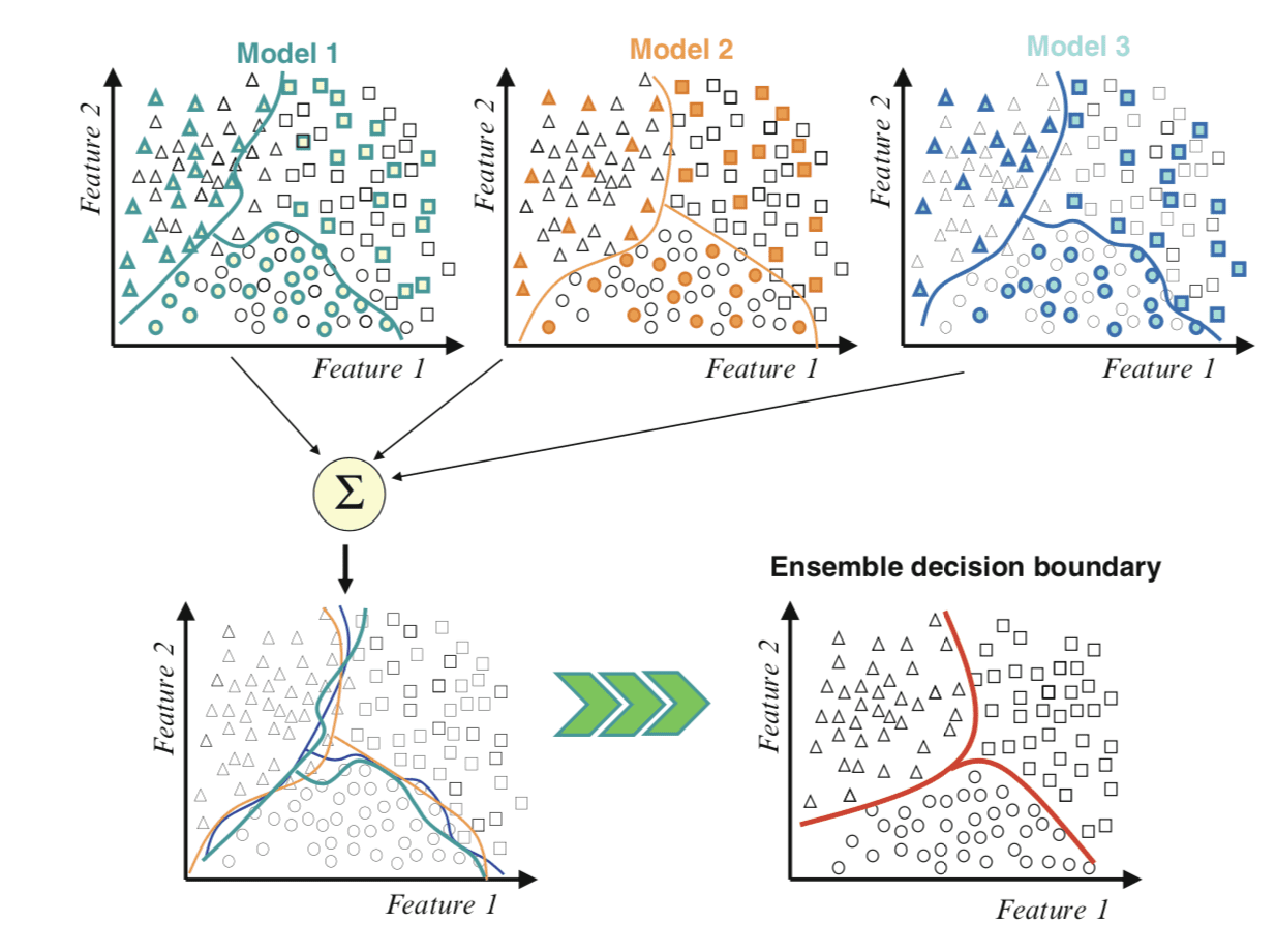
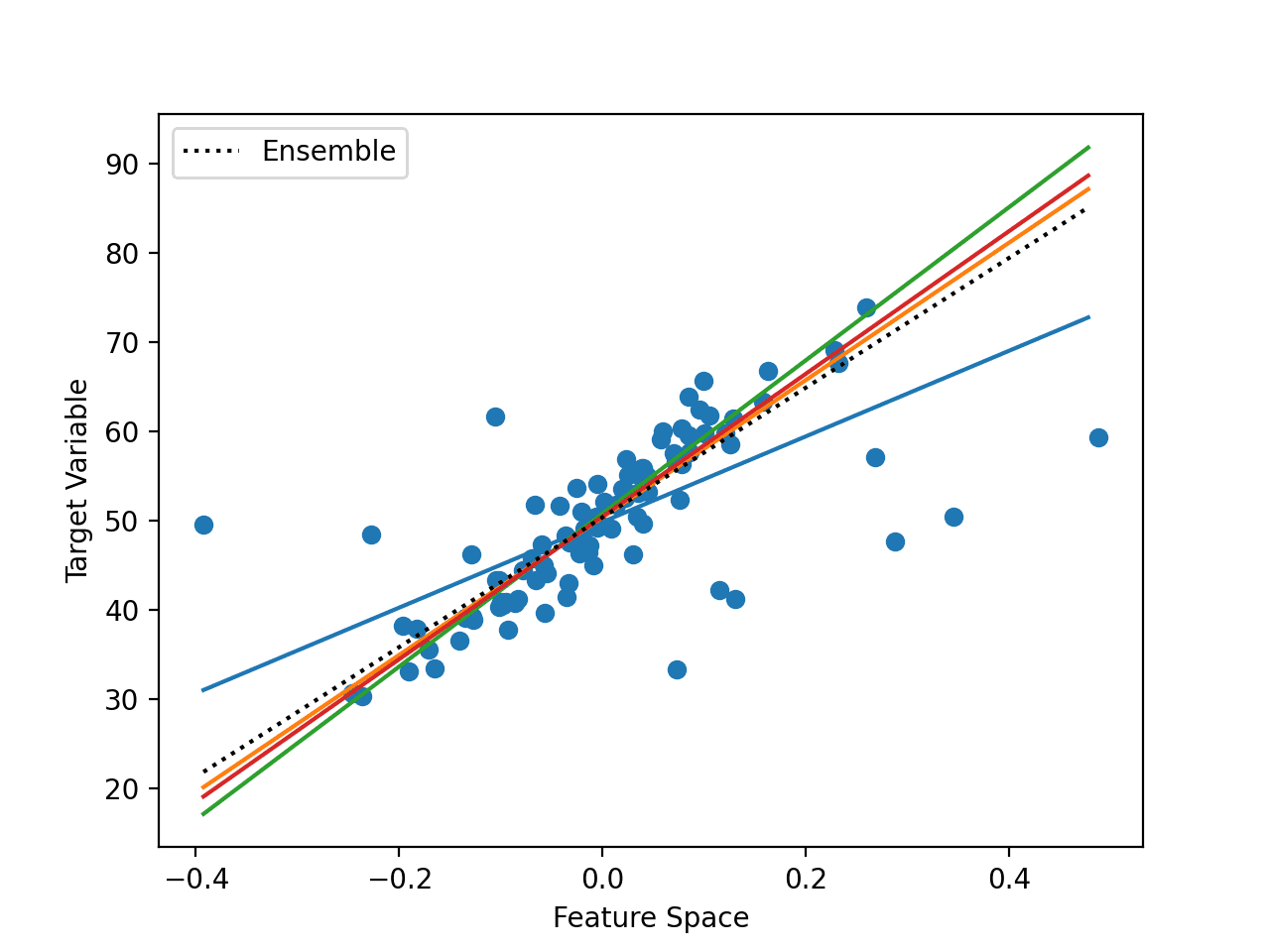
Blending is an ensemble machine learning technique that uses a machine learning model to learn how to best combine the predictions from multiple contributing ensemble member models.

As such, blending is the same as stacked generalization, known as stacking, broadly conceived. Often, blending and stacking are used interchangeably in the same paper or model description.

Many machine learning practitioners have had success using stacking and related techniques to boost prediction accuracy beyond the level obtained by any of the individual models. In some contexts, stacking is also referred to as blending, and we will use the terms interchangeably here.

— Feature-Weighted Linear Stacking, 2009.

The architecture of a stacking model involves two or more base models, often referred to as level-0 models, and a meta-model that combines the predictions of the base models, referred to as a level-1 model. The meta-model is trained on the predictions made by base models on out-of-sample data.

Level-0 Models (Base-Models): Models fit on the training data and whose predictions are compiled.
Level-1 Model (Meta-Model): Model that learns how to best combine the predictions of the base models.

Nevertheless, blending has specific connotations for how to construct a stacking ensemble model.

Blending may suggest developing a stacking ensemble where the base-models are machine learning models of any type, and the meta-model is a linear model that “blends” the predictions of the base-models.

For example, a linear regression model when predicting a numerical value or a logistic regression model when predicting a class label would calculate a weighted sum of the predictions made by base models and would be considered a blending of predictions.

Blending Ensemble: Use of a linear model, such as linear regression or logistic regression, as the meta-model in a stacking ensemble.

Blending was the term commonly used for stacking ensembles during the Netflix prize in 2009. The prize involved teams seeking movie recommendation predictions that performed better than the native Netflix algorithm and a US$1M prize was awarded to the team that achieved a 10 percent performance improvement.

Our RMSE=0.8643^2 solution is a linear blend of over 100 results. […] Throughout the description of the methods, we highlight the specific predictors that participated in the final blended solution.

— The BellKor 2008 Solution to the Netflix Prize, 2008.

As such, blending is a colloquial term for ensemble learning with a stacking-type architecture model. It is rarely, if ever, used in textbooks or academic papers, other than those related to competitive machine learning.

Most commonly, blending is used to describe the specific application of stacking where the meta-model is trained on the predictions made by base-models on a hold-out validation dataset. In this context, stacking is reserved for a meta-model that is trained on out-of fold predictions during a cross-validation procedure.

Blending: Stacking-type ensemble where the meta-model is trained on predictions made on a holdout dataset.
Stacking: Stacking-type ensemble where the meta-model is trained on out-of-fold predictions made during k-fold cross-validation.

This distinction is common among the Kaggle competitive machine learning community.

Blending is a word introduced by the Netflix winners. It is very close to stacked generalization, but a bit simpler and less risk of an information leak. […] With blending, instead of creating out-of-fold predictions for the train set, you create a small holdout set of say 10% of the train set. The stacker model then trains on this holdout set only.

— Kaggle Ensemble Guide, MLWave, 2015.

We will use this latter definition of blending.

Next, let’s look at how we can implement blending.

Develop a Blending Ensemble

The scikit-learn library does not natively support blending at the time of writing.

Instead, we can implement it ourselves using scikit-learn models.

First, we need to create a number of base models. These can be any models we like for a regression or classification problem. We can define a function get_models() that returns a list of models where each model is defined as a tuple with a name and the configured classifier or regression object.

For example, for a classification problem, we might use a logistic regression, kNN, decision tree, SVM, and Naive Bayes model.

# get a list of base models
def get_models():
	models = list()
	models.append(('lr', LogisticRegression()))
	models.append(('knn', KNeighborsClassifier()))
	models.append(('cart', DecisionTreeClassifier()))
	models.append(('svm', SVC(probability=True)))
	models.append(('bayes', GaussianNB()))
	return models

Next, we need to fit the blending model.

Recall that the base models are fit on a training dataset. The meta-model is fit on the predictions made by each base model on a holdout dataset.

First, we can enumerate the list of models and fit each in turn on the training dataset. Also in this loop, we can use the fit model to make a prediction on the hold out (validation) dataset and store the predictions for later.

...
# fit all models on the training set and predict on hold out set
meta_X = list()
for name, model in models:
	# fit in training set
	model.fit(X_train, y_train)
	# predict on hold out set
	yhat = model.predict(X_val)
	# reshape predictions into a matrix with one column
	yhat = yhat.reshape(len(yhat), 1)
	# store predictions as input for blending
	meta_X.append(yhat)

We now have “meta_X” that represents the input data that can be used to train the meta-model. Each column or feature represents the output of one base model.

Each row represents the one sample from the holdout dataset. We can use the hstack() function to ensure this dataset is a 2D numpy array as expected by a machine learning model.

...
# create 2d array from predictions, each set is an input feature
meta_X = hstack(meta_X)

We can now train our meta-model. This can be any machine learning model we like, such as logistic regression for classification.

...
# define blending model
blender = LogisticRegression()
# fit on predictions from base models
blender.fit(meta_X, y_val)

We can tie all of this together into a function named fit_ensemble() that trains the blending model using a training dataset and holdout validation dataset.

# fit the blending ensemble
def fit_ensemble(models, X_train, X_val, y_train, y_val):
	# fit all models on the training set and predict on hold out set
	meta_X = list()
	for name, model in models:
		# fit in training set
		model.fit(X_train, y_train)
		# predict on hold out set
		yhat = model.predict(X_val)
		# reshape predictions into a matrix with one column
		yhat = yhat.reshape(len(yhat), 1)
		# store predictions as input for blending
		meta_X.append(yhat)
	# create 2d array from predictions, each set is an input feature
	meta_X = hstack(meta_X)
	# define blending model
	blender = LogisticRegression()
	# fit on predictions from base models
	blender.fit(meta_X, y_val)
	return blender

The next step is to use the blending ensemble to make predictions on new data.

This is a two-step process. The first step is to use each base model to make a prediction. These predictions are then gathered together and used as input to the blending model to make the final prediction.

We can use the same looping structure as we did when training the model. That is, we can collect the predictions from each base model into a training dataset, stack the predictions together, and call predict() on the blender model with this meta-level dataset.

The predict_ensemble() function below implements this. Given the list of fit base models, the fit blender ensemble, and a dataset (such as a test dataset or new data), it will return a set of predictions for the dataset.

# make a prediction with the blending ensemble
def predict_ensemble(models, blender, X_test):
	# make predictions with base models
	meta_X = list()
	for name, model in models:
		# predict with base model
		yhat = model.predict(X_test)
		# reshape predictions into a matrix with one column
		yhat = yhat.reshape(len(yhat), 1)
		# store prediction
		meta_X.append(yhat)
	# create 2d array from predictions, each set is an input feature
	meta_X = hstack(meta_X)
	# predict
	return blender.predict(meta_X)

We now have all of the elements required to implement a blending ensemble for classification or regression predictive modeling problems

Blending Ensemble for Classification

In this section, we will look at using blending for a classification problem.

First, we can use the make_classification() function to create a synthetic binary classification problem with 10,000 examples and 20 input features.

The complete example is listed below.

# test classification dataset
from sklearn.datasets import make_classification
# define dataset
X, y = make_classification(n_samples=10000, n_features=20, n_informative=15, n_redundant=5, random_state=7)
# summarize the dataset
print(X.shape, y.shape)

Running the example creates the dataset and summarizes the shape of the input and output components.

(10000, 20) (10000,)

Next, we need to split the dataset up, first into train and test sets, and then the training set into a subset used to train the base models and a subset used to train the meta-model.

In this case, we will use a 50-50 split for the train and test sets, then use a 67-33 split for train and validation sets.

...
# split dataset into train and test sets
X_train_full, X_test, y_train_full, y_test = train_test_split(X, y, test_size=0.5, random_state=1)
# split training set into train and validation sets
X_train, X_val, y_train, y_val = train_test_split(X_train_full, y_train_full, test_size=0.33, random_state=1)
# summarize data split
print('Train: %s, Val: %s, Test: %s' % (X_train.shape, X_val.shape, X_test.shape))

We can then use the get_models() function from the previous section to create the classification models used in the ensemble.

The fit_ensemble() function can then be called to fit the blending ensemble on the train and validation datasets and the predict_ensemble() function can be used to make predictions on the holdout dataset.

...
# create the base models
models = get_models()
# train the blending ensemble
blender = fit_ensemble(models, X_train, X_val, y_train, y_val)
# make predictions on test set
yhat = predict_ensemble(models, blender, X_test)

Finally, we can evaluate the performance of the blending model by reporting the classification accuracy on the test dataset.

...
# evaluate predictions
score = accuracy_score(y_test, yhat)
print('Blending Accuracy: %.3f' % score)

Tying this all together, the complete example of evaluating a blending ensemble on the synthetic binary classification problem is listed below.

# blending ensemble for classification using hard voting
from numpy import hstack
from sklearn.datasets import make_classification
from sklearn.model_selection import train_test_split
from sklearn.metrics import accuracy_score
from sklearn.linear_model import LogisticRegression
from sklearn.neighbors import KNeighborsClassifier
from sklearn.tree import DecisionTreeClassifier
from sklearn.svm import SVC
from sklearn.naive_bayes import GaussianNB

# get the dataset
def get_dataset():
	X, y = make_classification(n_samples=10000, n_features=20, n_informative=15, n_redundant=5, random_state=7)
	return X, y

# get a list of base models
def get_models():
	models = list()
	models.append(('lr', LogisticRegression()))
	models.append(('knn', KNeighborsClassifier()))
	models.append(('cart', DecisionTreeClassifier()))
	models.append(('svm', SVC()))
	models.append(('bayes', GaussianNB()))
	return models

# fit the blending ensemble
def fit_ensemble(models, X_train, X_val, y_train, y_val):
	# fit all models on the training set and predict on hold out set
	meta_X = list()
	for name, model in models:
		# fit in training set
		model.fit(X_train, y_train)
		# predict on hold out set
		yhat = model.predict(X_val)
		# reshape predictions into a matrix with one column
		yhat = yhat.reshape(len(yhat), 1)
		# store predictions as input for blending
		meta_X.append(yhat)
	# create 2d array from predictions, each set is an input feature
	meta_X = hstack(meta_X)
	# define blending model
	blender = LogisticRegression()
	# fit on predictions from base models
	blender.fit(meta_X, y_val)
	return blender

# make a prediction with the blending ensemble
def predict_ensemble(models, blender, X_test):
	# make predictions with base models
	meta_X = list()
	for name, model in models:
		# predict with base model
		yhat = model.predict(X_test)
		# reshape predictions into a matrix with one column
		yhat = yhat.reshape(len(yhat), 1)
		# store prediction
		meta_X.append(yhat)
	# create 2d array from predictions, each set is an input feature
	meta_X = hstack(meta_X)
	# predict
	return blender.predict(meta_X)

# define dataset
X, y = get_dataset()
# split dataset into train and test sets
X_train_full, X_test, y_train_full, y_test = train_test_split(X, y, test_size=0.5, random_state=1)
# split training set into train and validation sets
X_train, X_val, y_train, y_val = train_test_split(X_train_full, y_train_full, test_size=0.33, random_state=1)
# summarize data split
print('Train: %s, Val: %s, Test: %s' % (X_train.shape, X_val.shape, X_test.shape))
# create the base models
models = get_models()
# train the blending ensemble
blender = fit_ensemble(models, X_train, X_val, y_train, y_val)
# make predictions on test set
yhat = predict_ensemble(models, blender, X_test)
# evaluate predictions
score = accuracy_score(y_test, yhat)
print('Blending Accuracy: %.3f' % (score*100))

Running the example first reports the shape of the train, validation, and test datasets, then the accuracy of the ensemble on the test dataset.

In this case, we can see that the blending ensemble achieved a classification accuracy of about 97.900 percent.

Train: (3350, 20), Val: (1650, 20), Test: (5000, 20)
Blending Accuracy: 97.900

In the previous example, crisp class label predictions were combined using the blending model. This is a type of hard voting.

An alternative is to have each model predict class probabilities and use the meta-model to blend the probabilities. This is a type of soft voting and can result in better performance in some cases.

First, we must configure the models to return probabilities, such as the SVM model.

# get a list of base models
def get_models():
	models = list()
	models.append(('lr', LogisticRegression()))
	models.append(('knn', KNeighborsClassifier()))
	models.append(('cart', DecisionTreeClassifier()))
	models.append(('svm', SVC(probability=True)))
	models.append(('bayes', GaussianNB()))
	return models

Next, we must change the base models to predict probabilities instead of crisp class labels.

This can be achieved by calling the predict_proba() function in the fit_ensemble() function when fitting the base models.

...
# fit all models on the training set and predict on hold out set
meta_X = list()
for name, model in models:
	# fit in training set
	model.fit(X_train, y_train)
	# predict on hold out set
	yhat = model.predict_proba(X_val)
	# store predictions as input for blending
	meta_X.append(yhat)

This means that the meta dataset used to train the meta-model will have n columns per classifier, where n is the number of classes in the prediction problem, two in our case.

We also need to change the predictions made by the base models when using the blending model to make predictions on new data.

...
# make predictions with base models
meta_X = list()
for name, model in models:
	# predict with base model
	yhat = model.predict_proba(X_test)
	# store prediction
	meta_X.append(yhat)

Tying this together, the complete example of using blending on predicted class probabilities for the synthetic binary classification problem is listed below.

# blending ensemble for classification using soft voting
from numpy import hstack
from sklearn.datasets import make_classification
from sklearn.model_selection import train_test_split
from sklearn.metrics import accuracy_score
from sklearn.linear_model import LogisticRegression
from sklearn.neighbors import KNeighborsClassifier
from sklearn.tree import DecisionTreeClassifier
from sklearn.svm import SVC
from sklearn.naive_bayes import GaussianNB

# get the dataset
def get_dataset():
	X, y = make_classification(n_samples=10000, n_features=20, n_informative=15, n_redundant=5, random_state=7)
	return X, y

# get a list of base models
def get_models():
	models = list()
	models.append(('lr', LogisticRegression()))
	models.append(('knn', KNeighborsClassifier()))
	models.append(('cart', DecisionTreeClassifier()))
	models.append(('svm', SVC(probability=True)))
	models.append(('bayes', GaussianNB()))
	return models

# fit the blending ensemble
def fit_ensemble(models, X_train, X_val, y_train, y_val):
	# fit all models on the training set and predict on hold out set
	meta_X = list()
	for name, model in models:
		# fit in training set
		model.fit(X_train, y_train)
		# predict on hold out set
		yhat = model.predict_proba(X_val)
		# store predictions as input for blending
		meta_X.append(yhat)
	# create 2d array from predictions, each set is an input feature
	meta_X = hstack(meta_X)
	# define blending model
	blender = LogisticRegression()
	# fit on predictions from base models
	blender.fit(meta_X, y_val)
	return blender

# make a prediction with the blending ensemble
def predict_ensemble(models, blender, X_test):
	# make predictions with base models
	meta_X = list()
	for name, model in models:
		# predict with base model
		yhat = model.predict_proba(X_test)
		# store prediction
		meta_X.append(yhat)
	# create 2d array from predictions, each set is an input feature
	meta_X = hstack(meta_X)
	# predict
	return blender.predict(meta_X)

# define dataset
X, y = get_dataset()
# split dataset into train and test sets
X_train_full, X_test, y_train_full, y_test = train_test_split(X, y, test_size=0.5, random_state=1)
# split training set into train and validation sets
X_train, X_val, y_train, y_val = train_test_split(X_train_full, y_train_full, test_size=0.33, random_state=1)
# summarize data split
print('Train: %s, Val: %s, Test: %s' % (X_train.shape, X_val.shape, X_test.shape))
# create the base models
models = get_models()
# train the blending ensemble
blender = fit_ensemble(models, X_train, X_val, y_train, y_val)
# make predictions on test set
yhat = predict_ensemble(models, blender, X_test)
# evaluate predictions
score = accuracy_score(y_test, yhat)
print('Blending Accuracy: %.3f' % (score*100))

Running the example first reports the shape of the train, validation, and test datasets, then the accuracy of the ensemble on the test dataset.

In this case, we can see that blending the class probabilities resulted in a lift in classification accuracy to about 98.240 percent.

Train: (3350, 20), Val: (1650, 20), Test: (5000, 20)
Blending Accuracy: 98.240

A blending ensemble is only effective if it is able to out-perform any single contributing model.

We can confirm this by evaluating each of the base models in isolation. Each base model can be fit on the entire training dataset (unlike the blending ensemble) and evaluated on the test dataset (just like the blending ensemble).

The example below demonstrates this, evaluating each base model in isolation.

# evaluate base models on the entire training dataset
from sklearn.datasets import make_classification
from sklearn.model_selection import train_test_split
from sklearn.metrics import accuracy_score
from sklearn.linear_model import LogisticRegression
from sklearn.neighbors import KNeighborsClassifier
from sklearn.tree import DecisionTreeClassifier
from sklearn.svm import SVC
from sklearn.naive_bayes import GaussianNB

# get the dataset
def get_dataset():
	X, y = make_classification(n_samples=10000, n_features=20, n_informative=15, n_redundant=5, random_state=7)
	return X, y

# get a list of base models
def get_models():
	models = list()
	models.append(('lr', LogisticRegression()))
	models.append(('knn', KNeighborsClassifier()))
	models.append(('cart', DecisionTreeClassifier()))
	models.append(('svm', SVC(probability=True)))
	models.append(('bayes', GaussianNB()))
	return models

# define dataset
X, y = get_dataset()
# split dataset into train and test sets
X_train_full, X_test, y_train_full, y_test = train_test_split(X, y, test_size=0.5, random_state=1)
# summarize data split
print('Train: %s, Test: %s' % (X_train_full.shape, X_test.shape))
# create the base models
models = get_models()
# evaluate standalone model
for name, model in models:
	# fit the model on the training dataset
	model.fit(X_train_full, y_train_full)
	# make a prediction on the test dataset
	yhat = model.predict(X_test)
	# evaluate the predictions
	score = accuracy_score(y_test, yhat)
	# report the score
	print('>%s Accuracy: %.3f' % (name, score*100))

Running the example first reports the shape of the full train and test datasets, then the accuracy of each base model on the test dataset.

In this case, we can see that all models perform worse than the blended ensemble.

Interestingly, we can see that the SVM comes very close to achieving an accuracy of 98.200 percent compared to 98.240 achieved with the blending ensemble.

Train: (5000, 20), Test: (5000, 20)
>lr Accuracy: 87.800
>knn Accuracy: 97.380
>cart Accuracy: 88.200
>svm Accuracy: 98.200
>bayes Accuracy: 87.300

We may choose to use a blending ensemble as our final model.

This involves fitting the ensemble on the entire training dataset and making predictions on new examples. Specifically, the entire training dataset is split onto train and validation sets to train the base and meta-models respectively, then the ensemble can be used to make a prediction.

The complete example of making a prediction on new data with a blending ensemble for classification is listed below.

# example of making a prediction with a blending ensemble for classification
from numpy import hstack
from sklearn.datasets import make_classification
from sklearn.model_selection import train_test_split
from sklearn.linear_model import LogisticRegression
from sklearn.neighbors import KNeighborsClassifier
from sklearn.tree import DecisionTreeClassifier
from sklearn.svm import SVC
from sklearn.naive_bayes import GaussianNB

# get the dataset
def get_dataset():
	X, y = make_classification(n_samples=10000, n_features=20, n_informative=15, n_redundant=5, random_state=7)
	return X, y

# get a list of base models
def get_models():
	models = list()
	models.append(('lr', LogisticRegression()))
	models.append(('knn', KNeighborsClassifier()))
	models.append(('cart', DecisionTreeClassifier()))
	models.append(('svm', SVC(probability=True)))
	models.append(('bayes', GaussianNB()))
	return models

# fit the blending ensemble
def fit_ensemble(models, X_train, X_val, y_train, y_val):
	# fit all models on the training set and predict on hold out set
	meta_X = list()
	for _, model in models:
		# fit in training set
		model.fit(X_train, y_train)
		# predict on hold out set
		yhat = model.predict_proba(X_val)
		# store predictions as input for blending
		meta_X.append(yhat)
	# create 2d array from predictions, each set is an input feature
	meta_X = hstack(meta_X)
	# define blending model
	blender = LogisticRegression()
	# fit on predictions from base models
	blender.fit(meta_X, y_val)
	return blender

# make a prediction with the blending ensemble
def predict_ensemble(models, blender, X_test):
	# make predictions with base models
	meta_X = list()
	for _, model in models:
		# predict with base model
		yhat = model.predict_proba(X_test)
		# store prediction
		meta_X.append(yhat)
	# create 2d array from predictions, each set is an input feature
	meta_X = hstack(meta_X)
	# predict
	return blender.predict(meta_X)

# define dataset
X, y = get_dataset()
# split dataset set into train and validation sets
X_train, X_val, y_train, y_val = train_test_split(X, y, test_size=0.33, random_state=1)
# summarize data split
print('Train: %s, Val: %s' % (X_train.shape, X_val.shape))
# create the base models
models = get_models()
# train the blending ensemble
blender = fit_ensemble(models, X_train, X_val, y_train, y_val)
# make a prediction on a new row of data
row = [-0.30335011, 2.68066314, 2.07794281, 1.15253537, -2.0583897, -2.51936601, 0.67513028, -3.20651939, -1.60345385, 3.68820714, 0.05370913, 1.35804433, 0.42011397, 1.4732839, 2.89997622, 1.61119399, 7.72630965, -2.84089477, -1.83977415, 1.34381989]
yhat = predict_ensemble(models, blender, [row])
# summarize prediction
print('Predicted Class: %d' % (yhat))

Running the example fits the blending ensemble model on the dataset and is then used to make a prediction on a new row of data, as we might when using the model in an application.

Train: (6700, 20), Val: (3300, 20)
Predicted Class: 1

Next, let’s explore how we might evaluate a blending ensemble for regression.

Blending Ensemble for Regression

In this section, we will look at using stacking for a regression problem.

First, we can use the make_regression() function to create a synthetic regression problem with 10,000 examples and 20 input features.

The complete example is listed below.

# test regression dataset
from sklearn.datasets import make_regression
# define dataset
X, y = make_regression(n_samples=10000, n_features=20, n_informative=10, noise=0.3, random_state=7)
# summarize the dataset
print(X.shape, y.shape)

Running the example creates the dataset and summarizes the shape of the input and output components.

(10000, 20) (10000,)

Next, we can define the list of regression models to use as base models. In this case, we will use linear regression, kNN, decision tree, and SVM models.

# get a list of base models
def get_models():
	models = list()
	models.append(('lr', LinearRegression()))
	models.append(('knn', KNeighborsRegressor()))
	models.append(('cart', DecisionTreeRegressor()))
	models.append(('svm', SVR()))
	return models

The fit_ensemble() function used to train the blending ensemble is unchanged from classification, other than the model used for blending must be changed to a regression model.

We will use the linear regression model in this case.

...
# define blending model
blender = LinearRegression()

Given that it is a regression problem, we will evaluate the performance of the model using an error metric, in this case, the mean absolute error, or MAE for short.

...
# evaluate predictions
score = mean_absolute_error(y_test, yhat)
print('Blending MAE: %.3f' % score)

Tying this together, the complete example of a blending ensemble for the synthetic regression predictive modeling problem is listed below.

# evaluate blending ensemble for regression
from numpy import hstack
from sklearn.datasets import make_regression
from sklearn.model_selection import train_test_split
from sklearn.metrics import mean_absolute_error
from sklearn.linear_model import LinearRegression
from sklearn.neighbors import KNeighborsRegressor
from sklearn.tree import DecisionTreeRegressor
from sklearn.svm import SVR

# get the dataset
def get_dataset():
	X, y = make_regression(n_samples=10000, n_features=20, n_informative=10, noise=0.3, random_state=7)
	return X, y

# get a list of base models
def get_models():
	models = list()
	models.append(('lr', LinearRegression()))
	models.append(('knn', KNeighborsRegressor()))
	models.append(('cart', DecisionTreeRegressor()))
	models.append(('svm', SVR()))
	return models

# fit the blending ensemble
def fit_ensemble(models, X_train, X_val, y_train, y_val):
	# fit all models on the training set and predict on hold out set
	meta_X = list()
	for name, model in models:
		# fit in training set
		model.fit(X_train, y_train)
		# predict on hold out set
		yhat = model.predict(X_val)
		# reshape predictions into a matrix with one column
		yhat = yhat.reshape(len(yhat), 1)
		# store predictions as input for blending
		meta_X.append(yhat)
	# create 2d array from predictions, each set is an input feature
	meta_X = hstack(meta_X)
	# define blending model
	blender = LinearRegression()
	# fit on predictions from base models
	blender.fit(meta_X, y_val)
	return blender

# make a prediction with the blending ensemble
def predict_ensemble(models, blender, X_test):
	# make predictions with base models
	meta_X = list()
	for name, model in models:
		# predict with base model
		yhat = model.predict(X_test)
		# reshape predictions into a matrix with one column
		yhat = yhat.reshape(len(yhat), 1)
		# store prediction
		meta_X.append(yhat)
	# create 2d array from predictions, each set is an input feature
	meta_X = hstack(meta_X)
	# predict
	return blender.predict(meta_X)

# define dataset
X, y = get_dataset()
# split dataset into train and test sets
X_train_full, X_test, y_train_full, y_test = train_test_split(X, y, test_size=0.5, random_state=1)
# split training set into train and validation sets
X_train, X_val, y_train, y_val = train_test_split(X_train_full, y_train_full, test_size=0.33, random_state=1)
# summarize data split
print('Train: %s, Val: %s, Test: %s' % (X_train.shape, X_val.shape, X_test.shape))
# create the base models
models = get_models()
# train the blending ensemble
blender = fit_ensemble(models, X_train, X_val, y_train, y_val)
# make predictions on test set
yhat = predict_ensemble(models, blender, X_test)
# evaluate predictions
score = mean_absolute_error(y_test, yhat)
print('Blending MAE: %.3f' % score)

Running the example first reports the shape of the train, validation, and test datasets, then the MAE of the ensemble on the test dataset.

In this case, we can see that the blending ensemble achieved a MAE of about 0.237 on the test dataset.

Train: (3350, 20), Val: (1650, 20), Test: (5000, 20)
Blending MAE: 0.237

As with classification, the blending ensemble is only useful if it performs better than any of the base models that contribute to the ensemble.

We can check this by evaluating each base model in isolation by first fitting it on the entire training dataset (unlike the blending ensemble) and making predictions on the test dataset (like the blending ensemble).

The example below evaluates each of the base models in isolation on the synthetic regression predictive modeling dataset.

# evaluate base models in isolation on the regression dataset
from numpy import hstack
from sklearn.datasets import make_regression
from sklearn.model_selection import train_test_split
from sklearn.metrics import mean_absolute_error
from sklearn.linear_model import LinearRegression
from sklearn.neighbors import KNeighborsRegressor
from sklearn.tree import DecisionTreeRegressor
from sklearn.svm import SVR

# get the dataset
def get_dataset():
	X, y = make_regression(n_samples=10000, n_features=20, n_informative=10, noise=0.3, random_state=7)
	return X, y

# get a list of base models
def get_models():
	models = list()
	models.append(('lr', LinearRegression()))
	models.append(('knn', KNeighborsRegressor()))
	models.append(('cart', DecisionTreeRegressor()))
	models.append(('svm', SVR()))
	return models

# define dataset
X, y = get_dataset()
# split dataset into train and test sets
X_train_full, X_test, y_train_full, y_test = train_test_split(X, y, test_size=0.5, random_state=1)
# summarize data split
print('Train: %s, Test: %s' % (X_train_full.shape, X_test.shape))
# create the base models
models = get_models()
# evaluate standalone model
for name, model in models:
	# fit the model on the training dataset
	model.fit(X_train_full, y_train_full)
	# make a prediction on the test dataset
	yhat = model.predict(X_test)
	# evaluate the predictions
	score = mean_absolute_error(y_test, yhat)
	# report the score
	print('>%s MAE: %.3f' % (name, score))

Running the example first reports the shape of the full train and test datasets, then the MAE of each base model on the test dataset.

In this case, we can see that indeed the linear regression model has performed slightly better than the blending ensemble, achieving a MAE of 0.236 as compared to 0.237 with the ensemble. This may be because of the way that the synthetic dataset was constructed.

Nevertheless, in this case, we would choose to use the linear regression model directly on this problem. This highlights the importance of checking the performance of the contributing models before adopting an ensemble model as the final model.

Train: (5000, 20), Test: (5000, 20)
>lr MAE: 0.236
>knn MAE: 100.169
>cart MAE: 133.744
>svm MAE: 138.195

Again, we may choose to use a blending ensemble as our final model for regression.

This involves fitting splitting the entire dataset into train and validation sets to fit the base and meta-models respectively, then the ensemble can be used to make a prediction for a new row of data.

The complete example of making a prediction on new data with a blending ensemble for regression is listed below.

# example of making a prediction with a blending ensemble for regression
from numpy import hstack
from sklearn.datasets import make_regression
from sklearn.model_selection import train_test_split
from sklearn.linear_model import LinearRegression
from sklearn.neighbors import KNeighborsRegressor
from sklearn.tree import DecisionTreeRegressor
from sklearn.svm import SVR

# get the dataset
def get_dataset():
	X, y = make_regression(n_samples=10000, n_features=20, n_informative=10, noise=0.3, random_state=7)
	return X, y

# get a list of base models
def get_models():
	models = list()
	models.append(('lr', LinearRegression()))
	models.append(('knn', KNeighborsRegressor()))
	models.append(('cart', DecisionTreeRegressor()))
	models.append(('svm', SVR()))
	return models

# fit the blending ensemble
def fit_ensemble(models, X_train, X_val, y_train, y_val):
	# fit all models on the training set and predict on hold out set
	meta_X = list()
	for _, model in models:
		# fit in training set
		model.fit(X_train, y_train)
		# predict on hold out set
		yhat = model.predict(X_val)
		# reshape predictions into a matrix with one column
		yhat = yhat.reshape(len(yhat), 1)
		# store predictions as input for blending
		meta_X.append(yhat)
	# create 2d array from predictions, each set is an input feature
	meta_X = hstack(meta_X)
	# define blending model
	blender = LinearRegression()
	# fit on predictions from base models
	blender.fit(meta_X, y_val)
	return blender

# make a prediction with the blending ensemble
def predict_ensemble(models, blender, X_test):
	# make predictions with base models
	meta_X = list()
	for _, model in models:
		# predict with base model
		yhat = model.predict(X_test)
		# reshape predictions into a matrix with one column
		yhat = yhat.reshape(len(yhat), 1)
		# store prediction
		meta_X.append(yhat)
	# create 2d array from predictions, each set is an input feature
	meta_X = hstack(meta_X)
	# predict
	return blender.predict(meta_X)

# define dataset
X, y = get_dataset()
# split dataset set into train and validation sets
X_train, X_val, y_train, y_val = train_test_split(X, y, test_size=0.33, random_state=1)
# summarize data split
print('Train: %s, Val: %s' % (X_train.shape, X_val.shape))
# create the base models
models = get_models()
# train the blending ensemble
blender = fit_ensemble(models, X_train, X_val, y_train, y_val)
# make a prediction on a new row of data
row = [-0.24038754, 0.55423865, -0.48979221, 1.56074459, -1.16007611, 1.10049103, 1.18385406, -1.57344162, 0.97862519, -0.03166643, 1.77099821, 1.98645499, 0.86780193, 2.01534177, 2.51509494, -1.04609004, -0.19428148, -0.05967386, -2.67168985, 1.07182911]
yhat = predict_ensemble(models, blender, [row])
# summarize prediction
print('Predicted: %.3f' % (yhat[0]))

Running the example fits the blending ensemble model on the dataset and is then used to make a prediction on a new row of data, as we might when using the model in an application.

Train: (6700, 20), Val: (3300, 20)
Predicted: 359.986

Summary

In this tutorial, you discovered how to develop and evaluate a blending ensemble in python.

Specifically, you learned:

Blending ensembles are a type of stacking where the meta-model is fit using predictions on a holdout validation dataset instead of out-of-fold predictions.
How to develop a blending ensemble, including functions for training the model and making predictions on new data.
How to evaluate blending ensembles for classification and regression predictive modeling problems.

Do you have any questions?
Ask your questions in the comments below and I will do my best to answer.

The post Blending Ensemble Machine Learning With Python appeared first on Machine Learning Mastery.

Genetic Programming (GP) is an algorithm for evolving programs to solve specific well-defined problems.

It is a type of automatic programming intended for challenging problems where the task is well defined and solutions can be checked easily at a low cost, although the search space of possible solutions is vast, and there is little intuition as to the best way to solve the problem.

This often includes open problems such as controller design, circuit design, as well as predictive modeling tasks such as feature selection, classification, and regression.

It can be difficult for a beginner to get started in the field as there is a vast amount of literature going back decades.

In this tutorial, you will discover the top books on genetic programming.

Let’s get started.

Books on Genetic Programming
Photo by Luca Temporelli some rights reserved.

Tutorial Overview

There are a number of books on genetic programming, which can be grouped by type.

We will explore the top books on genetic programming divided into three main groups; they are:

Genetic Programming (Koza)
Textbooks
Conference Proceedings

Genetic Programming (Koza)

John Koza is a computer scientist that studied under John Holland, the inventor of the genetic algorithm.

Koza is typically credited with unifying the nascent field of genetic programming in the late 1980s and early 1990s.

He is famous for his application of genetic algorithms towards circuit designs that resulted in new patentable inventions and describing genetic algorithms as being about to routinely generate “human competitive” results.

He wrote a series of four textbooks on genetic programming, as follows:

His most recent book, “Genetic Programming IV,” is an excellent place to get started.

A table at the beginning of the book summarizes the four key takeaways; they are:

1. Genetic programming now routinely delivers high-return human-competitive machine intelligence.
2. Genetic programming is an automated invention machine.
3. Genetic programming can automatically create a general solution to a problem in the form of a parameterized topology.
4. Genetic programming has delivered a progression of qualitatively more substantial results in synchrony with five approximately order-of-magnitude increases in the expenditure of computer time.

— Page 1, Genetic Programming IV: Routine Human-Competitive Machine Intelligence, 2003.

The table of contents for this book is as follows:

Chapter 01: Introduction
Chapter 02: Background on Genetic Programming
Chapter 03: Automatic Synthesis of Controllers
Chapter 04: Automatic Synthesis of Circuits
Chapter 05: Automatic Synthesis of Circuit Topology, Sizing, Placement, and Routing
Chapter 06: Automatic Synthesis of Antennas
Chapter 07: Automatic Synthesis of Genetic Networks
Chapter 08: Automatic Synthesis of Metabolic Pathways
Chapter 09: Automatic Synthesis of Parameterized Topologies for Controllers
Chapter 10: Automatic Synthesis of Parameterized Topologies for Circuits
Chapter 11: Automatic Synthesis of Parameterized Topologies with Conditional Developmental Operators for Circuits
Chapter 12: Automatic Synthesis of Improved Tuning Rules for PID Controllers
Chapter 13: Automatic Synthesis of Parameterized Topologies for Improved Controllers
Chapter 14: Reinvention of Negative Feedback
Chapter 15: Automated Reinvention of Six Post-2000 Patented Circuits
Chapter 16: Problems for Which Genetic Programming May Be Well Suited
Chapter 17: Parallel Implementation and Computer Time
Chapter 18: Historical Perspective on Moore’s Law and the Progression of Qualitatively More Substantial Results Produced by Genetic Programming
Chapter 19: Conclusion

Genetic Programming IV: Routine Human-Competitive Machine Intelligence

Textbooks

A number of textbooks have been published on genetic programming designed for undergraduate and postgraduate students interested in the field.

Perhaps the most popular books include the following:

Genetic Programming: An Introduction, 1997.
Genetic Programming and Data Structures, 1998.
Foundations of Genetic Programming, 2002.

I would recommend the more recent “Foundations of Genetic Programming.”

So Foundations of Genetic Programming should not be viewed only as a collection of techniques that one needs to know in order to be able to do GP well but also as a first attempt to chart and explore the mechanisms and fundamental principles behind genetic programming as a search algorithm. In writing this book we hoped to cast a tiny bit of light onto the theoretical foundations of Artificial Intelligence as a whole.

— Page IIX, Foundations of Genetic Programming, 2002.

The table of contents for this book is as follows:

Chapter 01: Introduction
Chapter 02: Fitness Landscapes
Chapter 03: Program Component Schema Theories
Chapter 04: Pessimistic GP Schema Theories
Chapter 05: Exact GP Schema Theorems
Chapter 06: Lessons from GP Schema Theory
Chapter 07: The Genetic Programming Search Space
Chapter 08: The GP Search Space: Theoretical Analysis
Chapter 09: Example I: The Artificial Ant
Chapter 10: Example II: The Max Problem
Chapter 11: GP Convergence and Bloat
Chapter 12: Conclusions

Foundations of Genetic Programming

Perhaps one of the more popular books on GP was self-published by top academics in the field and is intended for student and developers interested in applying genetic programming to their projects.

A Field Guide to Genetic Programming, 2008.

Here’s a snippet from the book:

Many books have been written which describe aspects of GP. Some provide general introductions to the field as a whole. However, no new introductory book on GP has been produced in the last decade, and anyone wanting to learn about GP is forced to map the terrain painfully on their own. This book attempts to fill that gap, by providing a modern field guide to GP for both newcomers and old-timers.

— A Field Guide to Genetic Programming, 2008.

The table of contents for this book is as follows:

Chapter 01: Introduction
Chapter 02: Representation, Initialization and Operations in Tree-based GP
Chapter 03: Getting Ready to Run Genetic Programming
Chapter 04: Example Genetic Programming Run
Chapter 05: Alternative Initializations and Operations in Tree-based GP
Chapter 06: Modular, Grammatical and Developmental Tree-based GP
Chapter 07: Linear and Graph Genetic Programming
Chapter 08: Probabilistic Genetic Programming
Chapter 09: Multi-objective Genetic Programming
Chapter 10: Fast and Distributed Genetic Programming
Chapter 11: GP Theory and its Applications
Chapter 12: Applications
Chapter 13: Troubleshooting GP
Chapter 14: Conclusions

A Field Guide to Genetic Programming

It is common to refer to versions of genetic programming algorithms specialized for different applications and representations by new names, such as “Linear Genetic Programming,” “Cartesian Genetic Programming,” and “Grammatical Evolution.”

Some textbooks on these specialized types of genetic programming algorithms include the following:

Linear Genetic Programming, 2006.
Cartesian Genetic Programming, 2011.
Grammatical Evolution: Evolutionary Automatic Programming in an Arbitrary Language, 2003.
Foundations in Grammatical Evolution for Dynamic Environments, 2009.
Handbook of Grammatical Evolution, 2018.

Handbook of Grammatical Evolution

Conference Proceedings

The main way that findings are shared in machine learning is via conferences, and conference proceedings provide a collection of top papers from a conference.

The papers presented at any given conference can jump around topics and be challenging to follow without some grounding in the field. Nevertheless, they can quickly get you up to speed with current and popular techniques.

I recommend focusing on the most recent issues of any proceedings. No need to go trawling back through the years.

There are three conference proceedings you may want to look at; they are:

Genetic Programming Theory and Practice
Genetic Programming European Conference
Advances in Genetic Programming

Let’s take a closer look at each in turn:

Genetic Programming Theory and Practice

The Genetic Programming Theory and Practice conference is held annually, and the proceedings are printed by Springer.

It is probably the premier conference on GP. It is up to issue 17 (XVII) at the time of writing.

The last three issues are as follows:

Genetic Programming Theory and Practice XV, 2018.
Genetic Programming Theory and Practice XVI, 2019.
Genetic Programming Theory and Practice XVII, 2020.

Genetic Programming Theory and Practice

Genetic Programming European Conference

The Genetic Programming European Conference, or EuroGP, is another major genetic programming conference.

Like Genetic Programming Theory and Practice, this conference and its published proceedings have been going for decades and are in their 23rd year at the time of writing.

The last three issues are as follows:

Genetic Programming: 21st European Conference, EuroGP 2018
Genetic Programming: 22nd European Conference, EuroGP 2019
Genetic Programming: 23rd European Conference, EuroGP 2020

Genetic Programming: 23rd European Conference

Advances in Genetic Programming

“Advances in Genetic Programming” is a volume published by MIT press containing collected papers.

It was only published three times in the mid to late 1990s. Nevertheless, the contents may be useful for developing a deeper understanding of the field.

Advances in Genetic Programming, 1994.
Advances in Genetic Programming 2, 1996.
Advances in Genetic Programming 3, 1999.

Advances in Genetic Programming 3

Recommended Books

I have read most of the books listed.

If you are looking to get a single book on genetic programming, I would recommend the following:

A Field Guide to Genetic Programming, 2008.

It will introduce the field and show you how to get results quickly.

If you are looking for a fuller library of books, I would recommend the following three:

Genetic Programming IV: Routine Human-Competitive Machine Intelligence, 2003.
Foundations of Genetic Programming, 2002.
A Field Guide to Genetic Programming, 2008.

I have these three on my bookshelf.

With these three books, you will have a solid theoretical foundation, an idea of how to apply the technique in practice, and an idea of the types of human competitive results that have been achieved and the algorithms used to achieve them.

Summary

In this tutorial, you discovered the top books on genetic programming.

Have you read any of the above books?
What did you think?

Did I miss your favorite book?
Let me know in the comments below.

The post Books on Genetic Programming appeared first on Machine Learning Mastery.

Deep learning neural network models are fit on training data using the stochastic gradient descent optimization algorithm.

Updates to the weights of the model are made, using the backpropagation of error algorithm. The combination of the optimization and weight update algorithm was carefully chosen and is the most efficient approach known to fit neural networks.

Nevertheless, it is possible to use alternate optimization algorithms to fit a neural network model to a training dataset. This can be a useful exercise to learn more about how neural networks function and the central nature of optimization in applied machine learning. It may also be required for neural networks with unconventional model architectures and non-differentiable transfer functions.

In this tutorial, you will discover how to manually optimize the weights of neural network models.

After completing this tutorial, you will know:

How to develop the forward inference pass for neural network models from scratch.
How to optimize the weights of a Perceptron model for binary classification.
How to optimize the weights of a Multilayer Perceptron model using stochastic hill climbing.

Let’s get started.

How to Manually Optimize Neural Network Models
Photo by Bureau of Land Management, some rights reserved.

Tutorial Overview

This tutorial is divided into three parts; they are:

Optimize Neural Networks
Optimize a Perceptron Model
Optimize a Multilayer Perceptron

Optimize Neural Networks

Deep learning or neural networks are a flexible type of machine learning.

They are models composed of nodes and layers inspired by the structure and function of the brain. A neural network model works by propagating a given input vector through one or more layers to produce a numeric output that can be interpreted for classification or regression predictive modeling.

Models are trained by repeatedly exposing the model to examples of input and output and adjusting the weights to minimize the error of the model’s output compared to the expected output. This is called the stochastic gradient descent optimization algorithm. The weights of the model are adjusted using a specific rule from calculus that assigns error proportionally to each weight in the network. This is called the backpropagation algorithm.

The stochastic gradient descent optimization algorithm with weight updates made using backpropagation is the best way to train neural network models. However, it is not the only way to train a neural network.

It is possible to use any arbitrary optimization algorithm to train a neural network model.

That is, we can define a neural network model architecture and use a given optimization algorithm to find a set of weights for the model that results in a minimum of prediction error or a maximum of classification accuracy.

Using alternate optimization algorithms is expected to be less efficient on average than using stochastic gradient descent with backpropagation. Nevertheless, it may be more efficient in some specific cases, such as non-standard network architectures or non-differential transfer functions.

It can also be an interesting exercise to demonstrate the central nature of optimization in training machine learning algorithms, and specifically neural networks.

Next, let’s explore how to train a simple one-node neural network called a Perceptron model using stochastic hill climbing.

Optimize a Perceptron Model

The Perceptron algorithm is the simplest type of artificial neural network.

It is a model of a single neuron that can be used for two-class classification problems and provides the foundation for later developing much larger networks.

In this section, we will optimize the weights of a Perceptron neural network model.

First, let’s define a synthetic binary classification problem that we can use as the focus of optimizing the model.

We can use the make_classification() function to define a binary classification problem with 1,000 rows and five input variables.

The example below creates the dataset and summarizes the shape of the data.

# define a binary classification dataset
from sklearn.datasets import make_classification
# define dataset
X, y = make_classification(n_samples=1000, n_features=5, n_informative=2, n_redundant=1, random_state=1)
# summarize the shape of the dataset
print(X.shape, y.shape)

Running the example prints the shape of the created dataset, confirming our expectations.

(1000, 5) (1000,)

Next, we need to define a Perceptron model.

The Perceptron model has a single node that has one input weight for each column in the dataset.

Each input is multiplied by its corresponding weight to give a weighted sum and a bias weight is then added, like an intercept coefficient in a regression model. This weighted sum is called the activation. Finally, the activation is interpreted and used to predict the class label, 1 for a positive activation and 0 for a negative activation.

Before we optimize the model weights, we must develop the model and our confidence in how it works.

Let’s start by defining a function for interpreting the activation of the model.

This is called the activation function, or the transfer function; the latter name is more traditional and is my preference.

The transfer() function below takes the activation of the model and returns a class label, class=1 for a positive or zero activation and class=0 for a negative activation. This is called a step transfer function.

# transfer function
def transfer(activation):
	if activation >= 0.0:
		return 1
	return 0

Next, we can develop a function that calculates the activation of the model for a given input row of data from the dataset.

This function will take the row of data and the weights for the model and calculate the weighted sum of the input with the addition of the bias weight. The activate() function below implements this.

Note: We are using simple Python lists and imperative programming style instead of NumPy arrays or list compressions intentionally to make the code more readable for Python beginners. Feel free to optimize it and post your code in the comments below.

# activation function
def activate(row, weights):
	# add the bias, the last weight
	activation = weights[-1]
	# add the weighted input
	for i in range(len(row)):
		activation += weights[i] * row[i]
	return activation

Next, we can use the activate() and transfer() functions together to generate a prediction for a given row of data. The predict_row() function below implements this.

# use model weights to predict 0 or 1 for a given row of data
def predict_row(row, weights):
	# activate for input
	activation = activate(row, weights)
	# transfer for activation
	return transfer(activation)

Next, we can call the predict_row() function for each row in a given dataset. The predict_dataset() function below implements this.

Again, we are intentionally using simple imperative coding style for readability instead of list compressions.

# use model weights to generate predictions for a dataset of rows
def predict_dataset(X, weights):
	yhats = list()
	for row in X:
		yhat = predict_row(row, weights)
		yhats.append(yhat)
	return yhats

Finally, we can use the model to make predictions on our synthetic dataset to confirm it is all working correctly.

We can generate a random set of model weights using the rand() function.

Recall that we need one weight for each input (five inputs in this dataset) plus an extra weight for the bias weight.

...
# define dataset
X, y = make_classification(n_samples=1000, n_features=5, n_informative=2, n_redundant=1, random_state=1)
# determine the number of weights
n_weights = X.shape[1] + 1
# generate random weights
weights = rand(n_weights)

We can then use these weights with the dataset to make predictions.

...
# generate predictions for dataset
yhat = predict_dataset(X, weights)

We can evaluate the classification accuracy of these predictions.

...
# calculate accuracy
score = accuracy_score(y, yhat)
print(score)

That’s it.

We can tie all of this together and demonstrate our simple Perceptron model for classification. The complete example is listed below.

# simple perceptron model for binary classification
from numpy.random import rand
from sklearn.datasets import make_classification
from sklearn.metrics import accuracy_score

# transfer function
def transfer(activation):
	if activation >= 0.0:
		return 1
	return 0

# activation function
def activate(row, weights):
	# add the bias, the last weight
	activation = weights[-1]
	# add the weighted input
	for i in range(len(row)):
		activation += weights[i] * row[i]
	return activation

# use model weights to predict 0 or 1 for a given row of data
def predict_row(row, weights):
	# activate for input
	activation = activate(row, weights)
	# transfer for activation
	return transfer(activation)

# use model weights to generate predictions for a dataset of rows
def predict_dataset(X, weights):
	yhats = list()
	for row in X:
		yhat = predict_row(row, weights)
		yhats.append(yhat)
	return yhats

# define dataset
X, y = make_classification(n_samples=1000, n_features=5, n_informative=2, n_redundant=1, random_state=1)
# determine the number of weights
n_weights = X.shape[1] + 1
# generate random weights
weights = rand(n_weights)
# generate predictions for dataset
yhat = predict_dataset(X, weights)
# calculate accuracy
score = accuracy_score(y, yhat)
print(score)

Running the example generates a prediction for each example in the training dataset then prints the classification accuracy for the predictions.

We would expect about 50 percent accuracy given a set of random weights and a dataset with an equal number of examples in each class, and that is approximately what we see in this case.

0.548

We can now optimize the weights of the dataset to achieve good accuracy on this dataset.

First, we need to split the dataset into train and test sets. It is important to hold back some data not used in optimizing the model so that we can prepare a reasonable estimate of the performance of the model when used to make predictions on new data.

We will use 67 percent of the data for training and the remaining 33 percent as a test set for evaluating the performance of the model.

...
# split into train test sets
X_train, X_test, y_train, y_test = train_test_split(X, y, test_size=0.33)

Next, we can develop a stochastic hill climbing algorithm.

The optimization algorithm requires an objective function to optimize. It must take a set of weights and return a score that is to be minimized or maximized corresponding to a better model.

In this case, we will evaluate the accuracy of the model with a given set of weights and return the classification accuracy, which must be maximized.

The objective() function below implements this, given the dataset and a set of weights, and returns the accuracy of the model

# objective function
def objective(X, y, weights):
	# generate predictions for dataset
	yhat = predict_dataset(X, weights)
	# calculate accuracy
	score = accuracy_score(y, yhat)
	return score

Next, we can define the stochastic hill climbing algorithm.

The algorithm will require an initial solution (e.g. random weights) and will iteratively keep making small changes to the solution and checking if it results in a better performing model. The amount of change made to the current solution is controlled by a step_size hyperparameter. This process will continue for a fixed number of iterations, also provided as a hyperparameter.

The hillclimbing() function below implements this, taking the dataset, objective function, initial solution, and hyperparameters as arguments and returns the best set of weights found and the estimated performance.

# hill climbing local search algorithm
def hillclimbing(X, y, objective, solution, n_iter, step_size):
	# evaluate the initial point
	solution_eval = objective(X, y, solution)
	# run the hill climb
	for i in range(n_iter):
		# take a step
		candidate = solution + randn(len(solution)) * step_size
		# evaluate candidate point
		candidte_eval = objective(X, y, candidate)
		# check if we should keep the new point
		if candidte_eval >= solution_eval:
			# store the new point
			solution, solution_eval = candidate, candidte_eval
			# report progress
			print('>%d %.5f' % (i, solution_eval))
	return [solution, solution_eval]

We can then call this function, passing in a set of weights as the initial solution and the training dataset as the dataset to optimize the model against.

...
# define the total iterations
n_iter = 1000
# define the maximum step size
step_size = 0.05
# determine the number of weights
n_weights = X.shape[1] + 1
# define the initial solution
solution = rand(n_weights)
# perform the hill climbing search
weights, score = hillclimbing(X_train, y_train, objective, solution, n_iter, step_size)
print('Done!')
print('f(%s) = %f' % (weights, score))

Finally, we can evaluate the best model on the test dataset and report the performance.

...
# generate predictions for the test dataset
yhat = predict_dataset(X_test, weights)
# calculate accuracy
score = accuracy_score(y_test, yhat)
print('Test Accuracy: %.5f' % (score * 100))

Tying this together, the complete example of optimizing the weights of a Perceptron model on the synthetic binary optimization dataset is listed below.

# hill climbing to optimize weights of a perceptron model for classification
from numpy import asarray
from numpy.random import randn
from numpy.random import rand
from sklearn.datasets import make_classification
from sklearn.model_selection import train_test_split
from sklearn.metrics import accuracy_score

# transfer function
def transfer(activation):
	if activation >= 0.0:
		return 1
	return 0

# activation function
def activate(row, weights):
	# add the bias, the last weight
	activation = weights[-1]
	# add the weighted input
	for i in range(len(row)):
		activation += weights[i] * row[i]
	return activation

# # use model weights to predict 0 or 1 for a given row of data
def predict_row(row, weights):
	# activate for input
	activation = activate(row, weights)
	# transfer for activation
	return transfer(activation)

# use model weights to generate predictions for a dataset of rows
def predict_dataset(X, weights):
	yhats = list()
	for row in X:
		yhat = predict_row(row, weights)
		yhats.append(yhat)
	return yhats

# objective function
def objective(X, y, weights):
	# generate predictions for dataset
	yhat = predict_dataset(X, weights)
	# calculate accuracy
	score = accuracy_score(y, yhat)
	return score

# hill climbing local search algorithm
def hillclimbing(X, y, objective, solution, n_iter, step_size):
	# evaluate the initial point
	solution_eval = objective(X, y, solution)
	# run the hill climb
	for i in range(n_iter):
		# take a step
		candidate = solution + randn(len(solution)) * step_size
		# evaluate candidate point
		candidte_eval = objective(X, y, candidate)
		# check if we should keep the new point
		if candidte_eval >= solution_eval:
			# store the new point
			solution, solution_eval = candidate, candidte_eval
			# report progress
			print('>%d %.5f' % (i, solution_eval))
	return [solution, solution_eval]

# define dataset
X, y = make_classification(n_samples=1000, n_features=5, n_informative=2, n_redundant=1, random_state=1)
# split into train test sets
X_train, X_test, y_train, y_test = train_test_split(X, y, test_size=0.33)
# define the total iterations
n_iter = 1000
# define the maximum step size
step_size = 0.05
# determine the number of weights
n_weights = X.shape[1] + 1
# define the initial solution
solution = rand(n_weights)
# perform the hill climbing search
weights, score = hillclimbing(X_train, y_train, objective, solution, n_iter, step_size)
print('Done!')
print('f(%s) = %f' % (weights, score))
# generate predictions for the test dataset
yhat = predict_dataset(X_test, weights)
# calculate accuracy
score = accuracy_score(y_test, yhat)
print('Test Accuracy: %.5f' % (score * 100))

Running the example will report the iteration number and classification accuracy each time there is an improvement made to the model.

At the end of the search, the performance of the best set of weights on the training dataset is reported and the performance of the same model on the test dataset is calculated and reported.

In this case, we can see that the optimization algorithm found a set of weights that achieved about 88.5 percent accuracy on the training dataset and about 81.8 percent accuracy on the test dataset.

...
>111 0.88060
>119 0.88060
>126 0.88209
>134 0.88209
>205 0.88209
>262 0.88209
>280 0.88209
>293 0.88209
>297 0.88209
>336 0.88209
>373 0.88209
>437 0.88358
>463 0.88507
>630 0.88507
>701 0.88507
Done!
f([ 0.0097317 0.13818088 1.17634326 -0.04296336 0.00485813 -0.14767616]) = 0.885075
Test Accuracy: 81.81818

Now that we are familiar with how to manually optimize the weights of a Perceptron model, let’s look at how we can extend the example to optimize the weights of a Multilayer Perceptron (MLP) model.

Optimize a Multilayer Perceptron

A Multilayer Perceptron (MLP) model is a neural network with one or more layers, where each layer has one or more nodes.

It is an extension of a Perceptron model and is perhaps the most widely used neural network (deep learning) model.

In this section, we will build on what we learned in the previous section to optimize the weights of MLP models with an arbitrary number of layers and nodes per layer.

First, we will develop the model and test it with random weights, then use stochastic hill climbing to optimize the model weights.

When using MLPs for binary classification, it is common to use a sigmoid transfer function (also called the logistic function) instead of the step transfer function used in the Perceptron.

This function outputs a real-value between 0-1 that represents a binomial probability distribution, e.g. the probability that an example belongs to class=1. The transfer() function below implements this.

# transfer function
def transfer(activation):
	# sigmoid transfer function
	return 1.0 / (1.0 + exp(-activation))

We can use the same activate() function from the previous section. Here, we will use it to calculate the activation for each node in a given layer.

The predict_row() function must be replaced with a more elaborate version.

The function takes a row of data and the network and returns the output of the network.

We will define our network as a list of lists. Each layer will be a list of nodes and each node will be a list or array of weights.

To calculate the prediction of the network, we simply enumerate the layers, then enumerate nodes, then calculate the activation and transfer output for each node. In this case, we will use the same transfer function for all nodes in the network, although this does not have to be the case.

For networks with more than one layer, the output from the previous layer is used as input to each node in the next layer. The output from the final layer in the network is then returned.

The predict_row() function below implements this.

# activation function for a network
def predict_row(row, network):
	inputs = row
	# enumerate the layers in the network from input to output
	for layer in network:
		new_inputs = list()
		# enumerate nodes in the layer
		for node in layer:
			# activate the node
			activation = activate(inputs, node)
			# transfer activation
			output = transfer(activation)
			# store output
			new_inputs.append(output)
		# output from this layer is input to the next layer
		inputs = new_inputs
	return inputs[0]

That’s about it.

Finally, we need to define a network to use.

For example, we can define an MLP with a single hidden layer with a single node as follows:

...
# create a one node network
node = rand(n_inputs + 1)
layer = [node]
network = [layer]

This is practically a Perceptron, although with a sigmoid transfer function. Quite boring.

Let’s define an MLP with one hidden layer and one output layer. The first hidden layer will have 10 nodes, and each node will take the input pattern from the dataset (e.g. five inputs). The output layer will have a single node that takes inputs from the outputs of the first hidden layer and then outputs a prediction.

...
# one hidden layer and an output layer
n_hidden = 10
hidden1 = [rand(n_inputs + 1) for _ in range(n_hidden)]
output1 = [rand(n_hidden + 1)]
network = [hidden1, output1]

We can then use the model to make predictions on the dataset.

...
# generate predictions for dataset
yhat = predict_dataset(X, network)

Before we calculate the classification accuracy, we must round the predictions to class labels 0 and 1.

...
# round the predictions
yhat = [round(y) for y in yhat]
# calculate accuracy
score = accuracy_score(y, yhat)
print(score)

Tying this all together, the complete example of evaluating an MLP with random initial weights on our synthetic binary classification dataset is listed below.

# develop an mlp model for classification
from math import exp
from numpy.random import rand
from sklearn.datasets import make_classification
from sklearn.metrics import accuracy_score

# transfer function
def transfer(activation):
	# sigmoid transfer function
	return 1.0 / (1.0 + exp(-activation))

# activation function
def activate(row, weights):
	# add the bias, the last weight
	activation = weights[-1]
	# add the weighted input
	for i in range(len(row)):
		activation += weights[i] * row[i]
	return activation

# activation function for a network
def predict_row(row, network):
	inputs = row
	# enumerate the layers in the network from input to output
	for layer in network:
		new_inputs = list()
		# enumerate nodes in the layer
		for node in layer:
			# activate the node
			activation = activate(inputs, node)
			# transfer activation
			output = transfer(activation)
			# store output
			new_inputs.append(output)
		# output from this layer is input to the next layer
		inputs = new_inputs
	return inputs[0]

# use model weights to generate predictions for a dataset of rows
def predict_dataset(X, network):
	yhats = list()
	for row in X:
		yhat = predict_row(row, network)
		yhats.append(yhat)
	return yhats

# define dataset
X, y = make_classification(n_samples=1000, n_features=5, n_informative=2, n_redundant=1, random_state=1)
# determine the number of inputs
n_inputs = X.shape[1]
# one hidden layer and an output layer
n_hidden = 10
hidden1 = [rand(n_inputs + 1) for _ in range(n_hidden)]
output1 = [rand(n_hidden + 1)]
network = [hidden1, output1]
# generate predictions for dataset
yhat = predict_dataset(X, network)
# round the predictions
yhat = [round(y) for y in yhat]
# calculate accuracy
score = accuracy_score(y, yhat)
print(score)

Running the example generates a prediction for each example in the training dataset, then prints the classification accuracy for the predictions.

Again, we would expect about 50 percent accuracy given a set of random weights and a dataset with an equal number of examples in each class, and that is approximately what we see in this case.

0.499

Next, we can apply the stochastic hill climbing algorithm to the dataset.

It is very much the same as applying hill climbing to the Perceptron model, except in this case, a step requires a modification to all weights in the network.

For this, we will develop a new function that creates a copy of the network and mutates each weight in the network while making the copy.

The step() function below implements this.

# take a step in the search space
def step(network, step_size):
	new_net = list()
	# enumerate layers in the network
	for layer in network:
		new_layer = list()
		# enumerate nodes in this layer
		for node in layer:
			# mutate the node
			new_node = node.copy() + randn(len(node)) * step_size
			# store node in layer
			new_layer.append(new_node)
		# store layer in network
		new_net.append(new_layer)
	return new_net

Modifying all weight in the network is aggressive.

A less aggressive step in the search space might be to make a small change to a subset of the weights in the model, perhaps controlled by a hyperparameter. This is left as an extension.

We can then call this new step() function from the hillclimbing() function.

# hill climbing local search algorithm
def hillclimbing(X, y, objective, solution, n_iter, step_size):
	# evaluate the initial point
	solution_eval = objective(X, y, solution)
	# run the hill climb
	for i in range(n_iter):
		# take a step
		candidate = step(solution, step_size)
		# evaluate candidate point
		candidte_eval = objective(X, y, candidate)
		# check if we should keep the new point
		if candidte_eval >= solution_eval:
			# store the new point
			solution, solution_eval = candidate, candidte_eval
			# report progress
			print('>%d %f' % (i, solution_eval))
	return [solution, solution_eval]

Tying this together, the complete example of applying stochastic hill climbing to optimize the weights of an MLP model for binary classification is listed below.

# stochastic hill climbing to optimize a multilayer perceptron for classification
from math import exp
from numpy.random import randn
from numpy.random import rand
from sklearn.datasets import make_classification
from sklearn.model_selection import train_test_split
from sklearn.metrics import accuracy_score

# transfer function
def transfer(activation):
	# sigmoid transfer function
	return 1.0 / (1.0 + exp(-activation))

# activation function
def activate(row, weights):
	# add the bias, the last weight
	activation = weights[-1]
	# add the weighted input
	for i in range(len(row)):
		activation += weights[i] * row[i]
	return activation

# activation function for a network
def predict_row(row, network):
	inputs = row
	# enumerate the layers in the network from input to output
	for layer in network:
		new_inputs = list()
		# enumerate nodes in the layer
		for node in layer:
			# activate the node
			activation = activate(inputs, node)
			# transfer activation
			output = transfer(activation)
			# store output
			new_inputs.append(output)
		# output from this layer is input to the next layer
		inputs = new_inputs
	return inputs[0]

# use model weights to generate predictions for a dataset of rows
def predict_dataset(X, network):
	yhats = list()
	for row in X:
		yhat = predict_row(row, network)
		yhats.append(yhat)
	return yhats

# objective function
def objective(X, y, network):
	# generate predictions for dataset
	yhat = predict_dataset(X, network)
	# round the predictions
	yhat = [round(y) for y in yhat]
	# calculate accuracy
	score = accuracy_score(y, yhat)
	return score

# take a step in the search space
def step(network, step_size):
	new_net = list()
	# enumerate layers in the network
	for layer in network:
		new_layer = list()
		# enumerate nodes in this layer
		for node in layer:
			# mutate the node
			new_node = node.copy() + randn(len(node)) * step_size
			# store node in layer
			new_layer.append(new_node)
		# store layer in network
		new_net.append(new_layer)
	return new_net

# hill climbing local search algorithm
def hillclimbing(X, y, objective, solution, n_iter, step_size):
	# evaluate the initial point
	solution_eval = objective(X, y, solution)
	# run the hill climb
	for i in range(n_iter):
		# take a step
		candidate = step(solution, step_size)
		# evaluate candidate point
		candidte_eval = objective(X, y, candidate)
		# check if we should keep the new point
		if candidte_eval >= solution_eval:
			# store the new point
			solution, solution_eval = candidate, candidte_eval
			# report progress
			print('>%d %f' % (i, solution_eval))
	return [solution, solution_eval]

# define dataset
X, y = make_classification(n_samples=1000, n_features=5, n_informative=2, n_redundant=1, random_state=1)
# split into train test sets
X_train, X_test, y_train, y_test = train_test_split(X, y, test_size=0.33)
# define the total iterations
n_iter = 1000
# define the maximum step size
step_size = 0.1
# determine the number of inputs
n_inputs = X.shape[1]
# one hidden layer and an output layer
n_hidden = 10
hidden1 = [rand(n_inputs + 1) for _ in range(n_hidden)]
output1 = [rand(n_hidden + 1)]
network = [hidden1, output1]
# perform the hill climbing search
network, score = hillclimbing(X_train, y_train, objective, network, n_iter, step_size)
print('Done!')
print('Best: %f' % (score))
# generate predictions for the test dataset
yhat = predict_dataset(X_test, network)
# round the predictions
yhat = [round(y) for y in yhat]
# calculate accuracy
score = accuracy_score(y_test, yhat)
print('Test Accuracy: %.5f' % (score * 100))

Running the example will report the iteration number and classification accuracy each time there is an improvement made to the model.

At the end of the search, the performance of the best set of weights on the training dataset is reported and the performance of the same model on the test dataset is calculated and reported.

In this case, we can see that the optimization algorithm found a set of weights that achieved about 87.3 percent accuracy on the training dataset and about 85.1 percent accuracy on the test dataset.

...
>55 0.755224
>56 0.765672
>59 0.794030
>66 0.805970
>77 0.835821
>120 0.838806
>165 0.840299
>188 0.841791
>218 0.846269
>232 0.852239
>237 0.852239
>239 0.855224
>292 0.867164
>368 0.868657
>823 0.868657
>852 0.871642
>889 0.871642
>892 0.871642
>992 0.873134
Done!
Best: 0.873134
Test Accuracy: 85.15152

Summary

In this tutorial, you discovered how to manually optimize the weights of neural network models.

Specifically, you learned:

How to develop the forward inference pass for neural network models from scratch.
How to optimize the weights of a Perceptron model for binary classification.
How to optimize the weights of a Multilayer Perceptron model using stochastic hill climbing.

Do you have any questions?
Ask your questions in the comments below and I will do my best to answer.

The post How to Manually Optimize Neural Network Models appeared first on Machine Learning Mastery.

Autoencoder is a type of neural network that can be used to learn a compressed representation of raw data.

An autoencoder is composed of an encoder and a decoder sub-models. The encoder compresses the input and the decoder attempts to recreate the input from the compressed version provided by the encoder. After training, the encoder model is saved and the decoder is discarded.

The encoder can then be used as a data preparation technique to perform feature extraction on raw data that can be used to train a different machine learning model.

In this tutorial, you will discover how to develop and evaluate an autoencoder for classification predictive modeling.

After completing this tutorial, you will know:

An autoencoder is a neural network model that can be used to learn a compressed representation of raw data.
How to train an autoencoder model on a training dataset and save just the encoder part of the model.
How to use the encoder as a data preparation step when training a machine learning model.

Let’s get started.

How to Develop an Autoencoder for Classification
Photo by Bernd Thaller, some rights reserved.

Tutorial Overview

This tutorial is divided into three parts; they are:

Autoencoders for Feature Extraction
Autoencoder for Classification
Encoder as Data Preparation for Predictive Model

Autoencoders for Feature Extraction

An autoencoder is a neural network model that seeks to learn a compressed representation of an input.

An autoencoder is a neural network that is trained to attempt to copy its input to its output.

— Page 502, Deep Learning, 2016.

They are an unsupervised learning method, although technically, they are trained using supervised learning methods, referred to as self-supervised.

Autoencoders are typically trained as part of a broader model that attempts to recreate the input.

For example:

X = model.predict(X)

The design of the autoencoder model purposefully makes this challenging by restricting the architecture to a bottleneck at the midpoint of the model, from which the reconstruction of the input data is performed.

There are many types of autoencoders, and their use varies, but perhaps the more common use is as a learned or automatic feature extraction model.

In this case, once the model is fit, the reconstruction aspect of the model can be discarded and the model up to the point of the bottleneck can be used. The output of the model at the bottleneck is a fixed-length vector that provides a compressed representation of the input data.

Usually they are restricted in ways that allow them to copy only approximately, and to copy only input that resembles the training data. Because the model is forced to prioritize which aspects of the input should be copied, it often learns useful properties of the data.

— Page 502, Deep Learning, 2016.

Input data from the domain can then be provided to the model and the output of the model at the bottleneck can be used as a feature vector in a supervised learning model, for visualization, or more generally for dimensionality reduction.

Next, let’s explore how we might develop an autoencoder for feature extraction on a classification predictive modeling problem.

Autoencoder for Classification

In this section, we will develop an autoencoder to learn a compressed representation of the input features for a classification predictive modeling problem.

First, let’s define a classification predictive modeling problem.

We will use the make_classification() scikit-learn function to define a synthetic binary (2-class) classification task with 100 input features (columns) and 1,000 examples (rows). Importantly, we will define the problem in such a way that most of the input variables are redundant (90 of the 100 or 90 percent), allowing the autoencoder later to learn a useful compressed representation.

The example below defines the dataset and summarizes its shape.

# synthetic classification dataset
from sklearn.datasets import make_classification
# define dataset
X, y = make_classification(n_samples=1000, n_features=100, n_informative=10, n_redundant=90, random_state=1)
# summarize the dataset
print(X.shape, y.shape)

Running the example defines the dataset and prints the shape of the arrays, confirming the number of rows and columns.

(1000, 100) (1000,)

Next, we will develop a Multilayer Perceptron (MLP) autoencoder model.

The model will take all of the input columns, then output the same values. It will learn to recreate the input pattern exactly.

The autoencoder consists of two parts: the encoder and the decoder. The encoder learns how to interpret the input and compress it to an internal representation defined by the bottleneck layer. The decoder takes the output of the encoder (the bottleneck layer) and attempts to recreate the input.

Once the autoencoder is trained, the decoder is discarded and we only keep the encoder and use it to compress examples of input to vectors output by the bottleneck layer.

In this first autoencoder, we won’t compress the input at all and will use a bottleneck layer the same size as the input. This should be an easy problem that the model will learn nearly perfectly and is intended to confirm our model is implemented correctly.

We will define the model using the functional API; if this is new to you, I recommend this tutorial:

How to Use the Keras Functional API for Deep Learning

Prior to defining and fitting the model, we will split the data into train and test sets and scale the input data by normalizing the values to the range 0-1, a good practice with MLPs.

...
# split into train test sets
X_train, X_test, y_train, y_test = train_test_split(X, y, test_size=0.33, random_state=1)
# scale data
t = MinMaxScaler()
t.fit(X_train)
X_train = t.transform(X_train)
X_test = t.transform(X_test)

We will define the encoder to have two hidden layers, the first with two times the number of inputs (e.g. 200) and the second with the same number of inputs (100), followed by the bottleneck layer with the same number of inputs as the dataset (100).

To ensure the model learns well, we will use batch normalization and leaky ReLU activation.

...
# define encoder
visible = Input(shape=(n_inputs,))
# encoder level 1
e = Dense(n_inputs*2)(visible)
e = BatchNormalization()(e)
e = LeakyReLU()(e)
# encoder level 2
e = Dense(n_inputs)(e)
e = BatchNormalization()(e)
e = LeakyReLU()(e)
# bottleneck
n_bottleneck = n_inputs
bottleneck = Dense(n_bottleneck)(e)

The decoder will be defined with a similar structure, although in reverse.

It will have two hidden layers, the first with the number of inputs in the dataset (e.g. 100) and the second with double the number of inputs (e.g. 200). The output layer will have the same number of nodes as there are columns in the input data and will use a linear activation function to output numeric values.

...
# define decoder, level 1
d = Dense(n_inputs)(bottleneck)
d = BatchNormalization()(d)
d = LeakyReLU()(d)
# decoder level 2
d = Dense(n_inputs*2)(d)
d = BatchNormalization()(d)
d = LeakyReLU()(d)
# output layer
output = Dense(n_inputs, activation='linear')(d)
# define autoencoder model
model = Model(inputs=visible, outputs=output)

The model will be fit using the efficient Adam version of stochastic gradient descent and minimizes the mean squared error, given that reconstruction is a type of multi-output regression problem.

...
# compile autoencoder model
model.compile(optimizer='adam', loss='mse')

We can plot the layers in the autoencoder model to get a feeling for how the data flows through the model.

...
# plot the autoencoder
plot_model(model, 'autoencoder_no_compress.png', show_shapes=True)

The image below shows a plot of the autoencoder.

Plot of Autoencoder Model for Classification With No Compression

Next, we can train the model to reproduce the input and keep track of the performance of the model on the hold-out test set.

...
# fit the autoencoder model to reconstruct input
history = model.fit(X_train, X_train, epochs=200, batch_size=16, verbose=2, validation_data=(X_test,X_test))

After training, we can plot the learning curves for the train and test sets to confirm the model learned the reconstruction problem well.

...
# plot loss
pyplot.plot(history.history['loss'], label='train')
pyplot.plot(history.history['val_loss'], label='test')
pyplot.legend()
pyplot.show()

Finally, we can save the encoder model for use later, if desired.

...
# define an encoder model (without the decoder)
encoder = Model(inputs=visible, outputs=bottleneck)
plot_model(encoder, 'encoder_no_compress.png', show_shapes=True)
# save the encoder to file
encoder.save('encoder.h5')

As part of saving the encoder, we will also plot the encoder model to get a feeling for the shape of the output of the bottleneck layer, e.g. a 100 element vector.

An example of this plot is provided below.

Plot of Encoder Model for Classification With No Compression

Tying this all together, the complete example of an autoencoder for reconstructing the input data for a classification dataset without any compression in the bottleneck layer is listed below.

# train autoencoder for classification with no compression in the bottleneck layer
from sklearn.datasets import make_classification
from sklearn.preprocessing import MinMaxScaler
from sklearn.model_selection import train_test_split
from tensorflow.keras.models import Model
from tensorflow.keras.layers import Input
from tensorflow.keras.layers import Dense
from tensorflow.keras.layers import LeakyReLU
from tensorflow.keras.layers import BatchNormalization
from tensorflow.keras.utils import plot_model
from matplotlib import pyplot
# define dataset
X, y = make_classification(n_samples=1000, n_features=100, n_informative=10, n_redundant=90, random_state=1)
# number of input columns
n_inputs = X.shape[1]
# split into train test sets
X_train, X_test, y_train, y_test = train_test_split(X, y, test_size=0.33, random_state=1)
# scale data
t = MinMaxScaler()
t.fit(X_train)
X_train = t.transform(X_train)
X_test = t.transform(X_test)
# define encoder
visible = Input(shape=(n_inputs,))
# encoder level 1
e = Dense(n_inputs*2)(visible)
e = BatchNormalization()(e)
e = LeakyReLU()(e)
# encoder level 2
e = Dense(n_inputs)(e)
e = BatchNormalization()(e)
e = LeakyReLU()(e)
# bottleneck
n_bottleneck = n_inputs
bottleneck = Dense(n_bottleneck)(e)
# define decoder, level 1
d = Dense(n_inputs)(bottleneck)
d = BatchNormalization()(d)
d = LeakyReLU()(d)
# decoder level 2
d = Dense(n_inputs*2)(d)
d = BatchNormalization()(d)
d = LeakyReLU()(d)
# output layer
output = Dense(n_inputs, activation='linear')(d)
# define autoencoder model
model = Model(inputs=visible, outputs=output)
# compile autoencoder model
model.compile(optimizer='adam', loss='mse')
# plot the autoencoder
plot_model(model, 'autoencoder_no_compress.png', show_shapes=True)
# fit the autoencoder model to reconstruct input
history = model.fit(X_train, X_train, epochs=200, batch_size=16, verbose=2, validation_data=(X_test,X_test))
# plot loss
pyplot.plot(history.history['loss'], label='train')
pyplot.plot(history.history['val_loss'], label='test')
pyplot.legend()
pyplot.show()
# define an encoder model (without the decoder)
encoder = Model(inputs=visible, outputs=bottleneck)
plot_model(encoder, 'encoder_no_compress.png', show_shapes=True)
# save the encoder to file
encoder.save('encoder.h5')

Running the example fits the model and reports loss on the train and test sets along the way.

Note: if you have problems creating the plots of the model, you can comment out the import and call the plot_model() function.

In this case, we see that loss gets low, but does not go to zero (as we might have expected) with no compression in the bottleneck layer. Perhaps further tuning the model architecture or learning hyperparameters is required.

...
42/42 - 0s - loss: 0.0032 - val_loss: 0.0016
Epoch 196/200
42/42 - 0s - loss: 0.0031 - val_loss: 0.0024
Epoch 197/200
42/42 - 0s - loss: 0.0032 - val_loss: 0.0015
Epoch 198/200
42/42 - 0s - loss: 0.0032 - val_loss: 0.0014
Epoch 199/200
42/42 - 0s - loss: 0.0031 - val_loss: 0.0020
Epoch 200/200
42/42 - 0s - loss: 0.0029 - val_loss: 0.0017

A plot of the learning curves is created showing that the model achieves a good fit in reconstructing the input, which holds steady throughout training, not overfitting.

Learning Curves of Training the Autoencoder Model Without Compression

So far, so good. We know how to develop an autoencoder without compression.

Next, let’s change the configuration of the model so that the bottleneck layer has half the number of nodes (e.g. 50).

...
# bottleneck
n_bottleneck = round(float(n_inputs) / 2.0)
bottleneck = Dense(n_bottleneck)(e)

Tying this together, the complete example is listed below.

# train autoencoder for classification with with compression in the bottleneck layer
from sklearn.datasets import make_classification
from sklearn.preprocessing import MinMaxScaler
from sklearn.model_selection import train_test_split
from tensorflow.keras.models import Model
from tensorflow.keras.layers import Input
from tensorflow.keras.layers import Dense
from tensorflow.keras.layers import LeakyReLU
from tensorflow.keras.layers import BatchNormalization
from tensorflow.keras.utils import plot_model
from matplotlib import pyplot
# define dataset
X, y = make_classification(n_samples=1000, n_features=100, n_informative=10, n_redundant=90, random_state=1)
# number of input columns
n_inputs = X.shape[1]
# split into train test sets
X_train, X_test, y_train, y_test = train_test_split(X, y, test_size=0.33, random_state=1)
# scale data
t = MinMaxScaler()
t.fit(X_train)
X_train = t.transform(X_train)
X_test = t.transform(X_test)
# define encoder
visible = Input(shape=(n_inputs,))
# encoder level 1
e = Dense(n_inputs*2)(visible)
e = BatchNormalization()(e)
e = LeakyReLU()(e)
# encoder level 2
e = Dense(n_inputs)(e)
e = BatchNormalization()(e)
e = LeakyReLU()(e)
# bottleneck
n_bottleneck = round(float(n_inputs) / 2.0)
bottleneck = Dense(n_bottleneck)(e)
# define decoder, level 1
d = Dense(n_inputs)(bottleneck)
d = BatchNormalization()(d)
d = LeakyReLU()(d)
# decoder level 2
d = Dense(n_inputs*2)(d)
d = BatchNormalization()(d)
d = LeakyReLU()(d)
# output layer
output = Dense(n_inputs, activation='linear')(d)
# define autoencoder model
model = Model(inputs=visible, outputs=output)
# compile autoencoder model
model.compile(optimizer='adam', loss='mse')
# plot the autoencoder
plot_model(model, 'autoencoder_compress.png', show_shapes=True)
# fit the autoencoder model to reconstruct input
history = model.fit(X_train, X_train, epochs=200, batch_size=16, verbose=2, validation_data=(X_test,X_test))
# plot loss
pyplot.plot(history.history['loss'], label='train')
pyplot.plot(history.history['val_loss'], label='test')
pyplot.legend()
pyplot.show()
# define an encoder model (without the decoder)
encoder = Model(inputs=visible, outputs=bottleneck)
plot_model(encoder, 'encoder_compress.png', show_shapes=True)
# save the encoder to file
encoder.save('encoder.h5')

Running the example fits the model and reports loss on the train and test sets along the way.

In this case, we see that loss gets similarly low as the above example without compression, suggesting that perhaps the model performs just as well with a bottleneck half the size.

...
42/42 - 0s - loss: 0.0029 - val_loss: 0.0010
Epoch 196/200
42/42 - 0s - loss: 0.0029 - val_loss: 0.0013
Epoch 197/200
42/42 - 0s - loss: 0.0030 - val_loss: 9.4472e-04
Epoch 198/200
42/42 - 0s - loss: 0.0028 - val_loss: 0.0015
Epoch 199/200
42/42 - 0s - loss: 0.0033 - val_loss: 0.0021
Epoch 200/200
42/42 - 0s - loss: 0.0027 - val_loss: 8.7731e-04

A plot of the learning curves is created, again showing that the model achieves a good fit in reconstructing the input, which holds steady throughout training, not overfitting.

Learning Curves of Training the Autoencoder Model With Compression

The trained encoder is saved to the file “encoder.h5” that we can load and use later.

Next, let’s explore how we might use the trained encoder model.

Encoder as Data Preparation for Predictive Model

In this section, we will use the trained encoder from the autoencoder to compress input data and train a different predictive model.

First, let’s establish a baseline in performance on this problem. This is important as if the performance of a model is not improved by the compressed encoding, then the compressed encoding does not add value to the project and should not be used.

We can train a logistic regression model on the training dataset directly and evaluate the performance of the model on the holdout test set.

The complete example is listed below.

# baseline in performance with logistic regression model
from sklearn.datasets import make_classification
from sklearn.preprocessing import MinMaxScaler
from sklearn.preprocessing import LabelEncoder
from sklearn.model_selection import train_test_split
from sklearn.linear_model import LogisticRegression
from sklearn.metrics import accuracy_score
# define dataset
X, y = make_classification(n_samples=1000, n_features=100, n_informative=10, n_redundant=90, random_state=1)
# split into train test sets
X_train, X_test, y_train, y_test = train_test_split(X, y, test_size=0.33, random_state=1)
# scale data
t = MinMaxScaler()
t.fit(X_train)
X_train = t.transform(X_train)
X_test = t.transform(X_test)
# define model
model = LogisticRegression()
# fit model on training set
model.fit(X_train, y_train)
# make prediction on test set
yhat = model.predict(X_test)
# calculate accuracy
acc = accuracy_score(y_test, yhat)
print(acc)

Running the example fits a logistic regression model on the training dataset and evaluates it on the test set.

In this case, we can see that the model achieves a classification accuracy of about 89.3 percent.

We would hope and expect that a logistic regression model fit on an encoded version of the input to achieve better accuracy for the encoding to be considered useful.

0.8939393939393939

We can update the example to first encode the data using the encoder model trained in the previous section.

First, we can load the trained encoder model from the file.

...
# load the model from file
encoder = load_model('encoder.h5')

We can then use the encoder to transform the raw input data (e.g. 100 columns) into bottleneck vectors (e.g. 50 element vectors).

This process can be applied to the train and test datasets.

...
# encode the train data
X_train_encode = encoder.predict(X_train)
# encode the test data
X_test_encode = encoder.predict(X_test)

We can then use this encoded data to train and evaluate the logistic regression model, as before.

...
# define the model
model = LogisticRegression()
# fit the model on the training set
model.fit(X_train_encode, y_train)
# make predictions on the test set
yhat = model.predict(X_test_encode)

Tying this together, the complete example is listed below.

# evaluate logistic regression on encoded input
from sklearn.datasets import make_classification
from sklearn.preprocessing import MinMaxScaler
from sklearn.preprocessing import LabelEncoder
from sklearn.model_selection import train_test_split
from sklearn.linear_model import LogisticRegression
from sklearn.metrics import accuracy_score
from tensorflow.keras.models import load_model
# define dataset
X, y = make_classification(n_samples=1000, n_features=100, n_informative=10, n_redundant=90, random_state=1)
# split into train test sets
X_train, X_test, y_train, y_test = train_test_split(X, y, test_size=0.33, random_state=1)
# scale data
t = MinMaxScaler()
t.fit(X_train)
X_train = t.transform(X_train)
X_test = t.transform(X_test)
# load the model from file
encoder = load_model('encoder.h5')
# encode the train data
X_train_encode = encoder.predict(X_train)
# encode the test data
X_test_encode = encoder.predict(X_test)
# define the model
model = LogisticRegression()
# fit the model on the training set
model.fit(X_train_encode, y_train)
# make predictions on the test set
yhat = model.predict(X_test_encode)
# calculate classification accuracy
acc = accuracy_score(y_test, yhat)
print(acc)

Running the example first encodes the dataset using the encoder, then fits a logistic regression model on the training dataset and evaluates it on the test set.

In this case, we can see that the model achieves a classification accuracy of about 93.9 percent.

This is a better classification accuracy than the same model evaluated on the raw dataset, suggesting that the encoding is helpful for our chosen model and test harness.

0.9393939393939394

Summary

In this tutorial, you discovered how to develop and evaluate an autoencoder for classification predictive modeling.

Specifically, you learned:

An autoencoder is a neural network model that can be used to learn a compressed representation of raw data.
How to train an autoencoder model on a training dataset and save just the encoder part of the model.
How to use the encoder as a data preparation step when training a machine learning model.

Do you have any questions?
Ask your questions in the comments below and I will do my best to answer.

The post Autoencoder Feature Extraction for Classification appeared first on Machine Learning Mastery.

Autoencoder is a type of neural network that can be used to learn a compressed representation of raw data.

An autoencoder is composed of encoder and a decoder sub-models. The encoder compresses the input and the decoder attempts to recreate the input from the compressed version provided by the encoder. After training, the encoder model is saved and the decoder is discarded.

The encoder can then be used as a data preparation technique to perform feature extraction on raw data that can be used to train a different machine learning model.

In this tutorial, you will discover how to develop and evaluate an autoencoder for regression predictive

After completing this tutorial, you will know:

An autoencoder is a neural network model that can be used to learn a compressed representation of raw data.
How to train an autoencoder model on a training dataset and save just the encoder part of the model.
How to use the encoder as a data preparation step when training a machine learning model.

Let’s get started.

Autoencoder Feature Extraction for Regression
Photo by Simon Matzinger, some rights reserved.

Tutorial Overview

This tutorial is divided into three parts; they are:

Autoencoders for Feature Extraction
Autoencoder for Regression
Autoencoder as Data Preparation

Autoencoders for Feature Extraction

An autoencoder is a neural network model that seeks to learn a compressed representation of an input.

An autoencoder is a neural network that is trained to attempt to copy its input to its output.

— Page 502, Deep Learning, 2016.

They are an unsupervised learning method, although technically, they are trained using supervised learning methods, referred to as self-supervised. They are typically trained as part of a broader model that attempts to recreate the input.

For example:

X = model.predict(X)

There are many types of autoencoders, and their use varies, but perhaps the more common use is as a learned or automatic feature extraction model.

In this case, once the model is fit, the reconstruction aspect of the model can be discarded and the model up to the point of the bottleneck can be used. The output of the model at the bottleneck is a fixed length vector that provides a compressed representation of the input data.

Usually they are restricted in ways that allow them to copy only approximately, and to copy only input that resembles the training data. Because the model is forced to prioritize which aspects of the input should be copied, it often learns useful properties of the data.

— Page 502, Deep Learning, 2016.

Next, let’s explore how we might develop an autoencoder for feature extraction on a regression predictive modeling problem.

Autoencoder for Regression

In this section, we will develop an autoencoder to learn a compressed representation of the input features for a regression predictive modeling problem.

First, let’s define a regression predictive modeling problem.

We will use the make_regression() scikit-learn function to define a synthetic regression task with 100 input features (columns) and 1,000 examples (rows). Importantly, we will define the problem in such a way that most of the input variables are redundant (90 of the 100 or 90 percent), allowing the autoencoder later to learn a useful compressed representation.

The example below defines the dataset and summarizes its shape.

# synthetic regression dataset
from sklearn.datasets import make_regression
# define dataset
X, y = make_regression(n_samples=1000, n_features=100, n_informative=10, noise=0.1, random_state=1)
# summarize the dataset
print(X.shape, y.shape)

Running the example defines the dataset and prints the shape of the arrays, confirming the number of rows and columns.

(1000, 100) (1000,)

Next, we will develop a Multilayer Perceptron (MLP) autoencoder model.

The model will take all of the input columns, then output the same values. It will learn to recreate the input pattern exactly.

Once the autoencoder is trained, the decode is discarded and we only keep the encoder and use it to compress examples of input to vectors output by the bottleneck layer.

We will define the model using the functional API. If this is new to you, I recommend this tutorial:

How to Use the Keras Functional API for Deep Learning

Prior to defining and fitting the model, we will split the data into train and test sets and scale the input data by normalizing the values to the range 0-1, a good practice with MLPs.

...
# split into train test sets
X_train, X_test, y_train, y_test = train_test_split(X, y, test_size=0.33, random_state=1)
# scale data
t = MinMaxScaler()
t.fit(X_train)
X_train = t.transform(X_train)
X_test = t.transform(X_test)

We will define the encoder to have one hidden layer with the same number of nodes as there are in the input data with batch normalization and ReLU activation.

This is followed by a bottleneck layer with the same number of nodes as columns in the input data, e.g. no compression.

...
# define encoder
visible = Input(shape=(n_inputs,))
e = Dense(n_inputs*2)(visible)
e = BatchNormalization()(e)
e = ReLU()(e)
# define bottleneck
n_bottleneck = n_inputs
bottleneck = Dense(n_bottleneck)(e)

The decoder will be defined with the same structure.

It will have one hidden layer with batch normalization and ReLU activation. The output layer will have the same number of nodes as there are columns in the input data and will use a linear activation function to output numeric values.

...
# define decoder
d = Dense(n_inputs*2)(bottleneck)
d = BatchNormalization()(d)
d = ReLU()(d)
# output layer
output = Dense(n_inputs, activation='linear')(d)
# define autoencoder model
model = Model(inputs=visible, outputs=output)
# compile autoencoder model
model.compile(optimizer='adam', loss='mse')

The model will be fit using the efficient Adam version of stochastic gradient descent and minimizes the mean squared error, given that reconstruction is a type of multi-output regression problem.

...
# compile autoencoder model
model.compile(optimizer='adam', loss='mse')

We can plot the layers in the autoencoder model to get a feeling for how the data flows through the model.

...
# plot the autoencoder
plot_model(model, 'autoencoder.png', show_shapes=True)

The image below shows a plot of the autoencoder.

Plot of the Autoencoder Model for Regression

Next, we can train the model to reproduce the input and keep track of the performance of the model on the holdout test set. The model is trained for 400 epochs and a batch size of 16 examples.

...
# fit the autoencoder model to reconstruct input
history = model.fit(X_train, X_train, epochs=400, batch_size=16, verbose=2, validation_data=(X_test,X_test))

After training, we can plot the learning curves for the train and test sets to confirm the model learned the reconstruction problem well.

...
# plot loss
pyplot.plot(history.history['loss'], label='train')
pyplot.plot(history.history['val_loss'], label='test')
pyplot.legend()
pyplot.show()

Finally, we can save the encoder model for use later, if desired.

...
# define an encoder model (without the decoder)
encoder = Model(inputs=visible, outputs=bottleneck)
plot_model(encoder, 'encoder.png', show_shapes=True)
# save the encoder to file
encoder.save('encoder.h5')

As part of saving the encoder, we will also plot the model to get a feeling for the shape of the output of the bottleneck layer, e.g. a 100-element vector.

An example of this plot is provided below.

Plot of Encoder Model for Regression With No Compression

Tying this all together, the complete example of an autoencoder for reconstructing the input data for a regression dataset without any compression in the bottleneck layer is listed below.

# train autoencoder for regression with no compression in the bottleneck layer
from sklearn.datasets import make_regression
from sklearn.preprocessing import MinMaxScaler
from sklearn.model_selection import train_test_split
from tensorflow.keras.models import Model
from tensorflow.keras.layers import Input
from tensorflow.keras.layers import Dense
from tensorflow.keras.layers import ReLU
from tensorflow.keras.layers import BatchNormalization
from tensorflow.keras.utils import plot_model
from matplotlib import pyplot
# define dataset
X, y = make_regression(n_samples=1000, n_features=100, n_informative=10, noise=0.1, random_state=1)
# number of input columns
n_inputs = X.shape[1]
# split into train test sets
X_train, X_test, y_train, y_test = train_test_split(X, y, test_size=0.33, random_state=1)
# scale data
t = MinMaxScaler()
t.fit(X_train)
X_train = t.transform(X_train)
X_test = t.transform(X_test)
# define encoder
visible = Input(shape=(n_inputs,))
e = Dense(n_inputs*2)(visible)
e = BatchNormalization()(e)
e = ReLU()(e)
# define bottleneck
n_bottleneck = n_inputs
bottleneck = Dense(n_bottleneck)(e)
# define decoder
d = Dense(n_inputs*2)(bottleneck)
d = BatchNormalization()(d)
d = ReLU()(d)
# output layer
output = Dense(n_inputs, activation='linear')(d)
# define autoencoder model
model = Model(inputs=visible, outputs=output)
# compile autoencoder model
model.compile(optimizer='adam', loss='mse')
# plot the autoencoder
plot_model(model, 'autoencoder.png', show_shapes=True)
# fit the autoencoder model to reconstruct input
history = model.fit(X_train, X_train, epochs=400, batch_size=16, verbose=2, validation_data=(X_test,X_test))
# plot loss
pyplot.plot(history.history['loss'], label='train')
pyplot.plot(history.history['val_loss'], label='test')
pyplot.legend()
pyplot.show()
# define an encoder model (without the decoder)
encoder = Model(inputs=visible, outputs=bottleneck)
plot_model(encoder, 'encoder.png', show_shapes=True)
# save the encoder to file
encoder.save('encoder.h5')

Running the example fits the model and reports loss on the train and test sets along the way.

Note: if you have problems creating the plots of the model, you can comment out the import and call the plot_model() function.

In this case, we see that loss gets low but does not go to zero (as we might have expected) with no compression in the bottleneck layer. Perhaps further tuning the model architecture or learning hyperparameters is required.

...
Epoch 393/400
42/42 - 0s - loss: 0.0025 - val_loss: 0.0024
Epoch 394/400
42/42 - 0s - loss: 0.0025 - val_loss: 0.0021
Epoch 395/400
42/42 - 0s - loss: 0.0023 - val_loss: 0.0021
Epoch 396/400
42/42 - 0s - loss: 0.0025 - val_loss: 0.0023
Epoch 397/400
42/42 - 0s - loss: 0.0024 - val_loss: 0.0022
Epoch 398/400
42/42 - 0s - loss: 0.0025 - val_loss: 0.0021
Epoch 399/400
42/42 - 0s - loss: 0.0026 - val_loss: 0.0022
Epoch 400/400
42/42 - 0s - loss: 0.0025 - val_loss: 0.0024

A plot of the learning curves is created showing that the model achieves a good fit in reconstructing the input, which holds steady throughout training, not overfitting.

Learning Curves of Training the Autoencoder Model for Regression Without Compression

So far, so good. We know how to develop an autoencoder without compression.

The trained encoder is saved to the file “encoder.h5” that we can load and use later.

Next, let’s explore how we might use the trained encoder model.

Autoencoder as Data Preparation

In this section, we will use the trained encoder model from the autoencoder model to compress input data and train a different predictive model.

We can train a support vector regression (SVR) model on the training dataset directly and evaluate the performance of the model on the holdout test set.

As is good practice, we will scale both the input variables and target variable prior to fitting and evaluating the model.

The complete example is listed below.

# baseline in performance with support vector regression model
from sklearn.datasets import make_regression
from sklearn.preprocessing import MinMaxScaler
from sklearn.model_selection import train_test_split
from sklearn.svm import SVR
from sklearn.metrics import mean_absolute_error
# define dataset
X, y = make_regression(n_samples=1000, n_features=100, n_informative=10, noise=0.1, random_state=1)
# split into train test sets
X_train, X_test, y_train, y_test = train_test_split(X, y, test_size=0.33, random_state=1)
# reshape target variables so that we can transform them
y_train = y_train.reshape((len(y_train), 1))
y_test = y_test.reshape((len(y_test), 1))
# scale input data
trans_in = MinMaxScaler()
trans_in.fit(X_train)
X_train = trans_in.transform(X_train)
X_test = trans_in.transform(X_test)
# scale output data
trans_out = MinMaxScaler()
trans_out.fit(y_train)
y_train = trans_out.transform(y_train)
y_test = trans_out.transform(y_test)
# define model
model = SVR()
# fit model on the training dataset
model.fit(X_train, y_train)
# make prediction on test set
yhat = model.predict(X_test)
# invert transforms so we can calculate errors
yhat = yhat.reshape((len(yhat), 1))
yhat = trans_out.inverse_transform(yhat)
y_test = trans_out.inverse_transform(y_test)
# calculate error
score = mean_absolute_error(y_test, yhat)
print(score)

Running the example fits an SVR model on the training dataset and evaluates it on the test set.

In this case, we can see that the model achieves a mean absolute error (MAE) of about 89.

We would hope and expect that a SVR model fit on an encoded version of the input to achieve lower error for the encoding to be considered useful.

89.51082036130629

We can update the example to first encode the data using the encoder model trained in the previous section.

First, we can load the trained encoder model from the file.

...
# load the model from file
encoder = load_model('encoder.h5')

We can then use the encoder to transform the raw input data (e.g. 100 columns) into bottleneck vectors (e.g. 100 element vectors).

This process can be applied to the train and test datasets.

...
# encode the train data
X_train_encode = encoder.predict(X_train)
# encode the test data
X_test_encode = encoder.predict(X_test)

We can then use this encoded data to train and evaluate the SVR model, as before.

...
# define model
model = SVR()
# fit model on the training dataset
model.fit(X_train_encode, y_train)
# make prediction on test set
yhat = model.predict(X_test_encode)

Tying this together, the complete example is listed below.

# support vector regression performance with encoded input
from sklearn.datasets import make_regression
from sklearn.preprocessing import MinMaxScaler
from sklearn.model_selection import train_test_split
from sklearn.svm import SVR
from sklearn.metrics import mean_absolute_error
from tensorflow.keras.models import load_model
# define dataset
X, y = make_regression(n_samples=1000, n_features=100, n_informative=10, noise=0.1, random_state=1)
# split into train test sets
X_train, X_test, y_train, y_test = train_test_split(X, y, test_size=0.33, random_state=1)
# reshape target variables so that we can transform them
y_train = y_train.reshape((len(y_train), 1))
y_test = y_test.reshape((len(y_test), 1))
# scale input data
trans_in = MinMaxScaler()
trans_in.fit(X_train)
X_train = trans_in.transform(X_train)
X_test = trans_in.transform(X_test)
# scale output data
trans_out = MinMaxScaler()
trans_out.fit(y_train)
y_train = trans_out.transform(y_train)
y_test = trans_out.transform(y_test)
# load the model from file
encoder = load_model('encoder.h5')
# encode the train data
X_train_encode = encoder.predict(X_train)
# encode the test data
X_test_encode = encoder.predict(X_test)
# define model
model = SVR()
# fit model on the training dataset
model.fit(X_train_encode, y_train)
# make prediction on test set
yhat = model.predict(X_test_encode)
# invert transforms so we can calculate errors
yhat = yhat.reshape((len(yhat), 1))
yhat = trans_out.inverse_transform(yhat)
y_test = trans_out.inverse_transform(y_test)
# calculate error
score = mean_absolute_error(y_test, yhat)
print(score)

Running the example first encodes the dataset using the encoder, then fits an SVR model on the training dataset and evaluates it on the test set.

In this case, we can see that the model achieves a MAE of about 69.

This is a better MAE than the same model evaluated on the raw dataset, suggesting that the encoding is helpful for our chosen model and test harness.

69.45890939600503

Summary

In this tutorial, you discovered how to develop and evaluate an autoencoder for regression predictive modeling.

Specifically, you learned:

An autoencoder is a neural network model that can be used to learn a compressed representation of raw data.
How to train an autoencoder model on a training dataset and save just the encoder part of the model.
How to use the encoder as a data preparation step when training a machine learning model.

Do you have any questions?
Ask your questions in the comments below and I will do my best to answer.

The post Autoencoder Feature Extraction for Regression appeared first on Machine Learning Mastery.

What are the Benefits of Ensemble Methods for Machine Learning?

Tutorial Overview

Ensemble Learning

Use Ensembles to Improve Robustness

Bias, Variance, and Ensembles

Use Ensembles to Improve Performance

Further Reading

Related Tutorials

Books

Articles

Summary

Tutorial Overview

Error-Correcting Output Codes

Evaluate and Use ECOC Classifiers

Tune Number of Bits Per Class

Further Reading

Related Tutorials

Papers

Books

APIs

Summary

Tutorial Overview

Random Subspace Ensemble

Random Subspace Ensemble via Bagging

Random Subspace Ensemble for Classification

Random Subspace Ensemble for Regression

Random Subspace Ensemble Hyperparameters

Explore Number of Trees

Explore Number of Features

Explore Alternate Algorithm

Further Reading

Papers

Books

APIs

Articles

Summary

Tutorial Overview

Random Forest Ensemble

Time Series Data Preparation

Random Forest for Time Series

Further Reading

Tutorials

APIs

Summary

Tutorial Overview

Curve Fitting

Curve Fitting Python API

Curve Fitting Worked Example

Further Reading

Books

APIs

Articles

Summary

Tutorial Overview

Hill Climbing Algorithm

Hill Climbing Algorithm Implementation

Example of Applying the Hill Climbing Algorithm

Further Reading

Tutorials

Books

APIs

Articles

Summary

Tutorial Overview

How Do Ensembles Work

Intuition for Classification Ensembles

Intuition for Regression Ensembles

Further Reading

Books

Articles

Summary

Tutorial Overview

What Is Overfitting

How to Perform an Overfitting Analysis

Example of Overfitting in Scikit-Learn

Counterexample of Overfitting in Scikit-Learn

Separate Overfitting Analysis From Model Selection

Further Reading

Tutorials

APIs