Quantcast
Channel: MachineLearningMastery.com
Viewing all 905 articles
Browse latest View live

Train-Test Split for Evaluating Machine Learning Algorithms

$
0
0

The train-test split procedure is used to estimate the performance of machine learning algorithms when they are used to make predictions on data not used to train the model.

It is a fast and easy procedure to perform, the results of which allow you to compare the performance of machine learning algorithms for your predictive modeling problem. Although simple to use and interpret, there are times when the procedure should not be used, such as when you have a small dataset and situations where additional configuration is required, such as when it is used for classification and the dataset is not balanced.

In this tutorial, you will discover how to evaluate machine learning models using the train-test split.

After completing this tutorial, you will know:

  • The train-test split procedure is appropriate when you have a very large dataset, a costly model to train, or require a good estimate of model performance quickly.
  • How to use the scikit-learn machine learning library to perform the train-test split procedure.
  • How to evaluate machine learning algorithms for classification and regression using the train-test split.

Let’s get started.

Train-Test Split for Evaluating Machine Learning Algorithms

Train-Test Split for Evaluating Machine Learning Algorithms
Photo by Paul VanDerWerf, some rights reserved.

Tutorial Overview

This tutorial is divided into three parts; they are:

  1. Train-Test Split Evaluation
    1. When to Use the Train-Test Split
    2. How to Configure the Train-Test Split
  2. Train-Test Split Procedure in Scikit-Learn
    1. Repeatable Train-Test Splits
    2. Stratified Train-Test Splits
  3. Train-Test Split to Evaluate Machine Learning Models
    1. Train-Test Split for Classification
    2. Train-Test Split for Regression

Train-Test Split Evaluation

The train-test split is a technique for evaluating the performance of a machine learning algorithm.

It can be used for classification or regression problems and can be used for any supervised learning algorithm.

The procedure involves taking a dataset and dividing it into two subsets. The first subset is used to fit the model and is referred to as the training dataset. The second subset is not used to train the model; instead, the input element of the dataset is provided to the model, then predictions are made and compared to the expected values. This second dataset is referred to as the test dataset.

  • Train Dataset: Used to fit the machine learning model.
  • Test Dataset: Used to evaluate the fit machine learning model.

The objective is to estimate the performance of the machine learning model on new data: data not used to train the model.

This is how we expect to use the model in practice. Namely, to fit it on available data with known inputs and outputs, then make predictions on new examples in the future where we do not have the expected output or target values.

The train-test procedure is appropriate when there is a sufficiently large dataset available.

When to Use the Train-Test Split

The idea of “sufficiently large” is specific to each predictive modeling problem. It means that there is enough data to split the dataset into train and test datasets and each of the train and test datasets are suitable representations of the problem domain. This requires that the original dataset is also a suitable representation of the problem domain.

A suitable representation of the problem domain means that there are enough records to cover all common cases and most uncommon cases in the domain. This might mean combinations of input variables observed in practice. It might require thousands, hundreds of thousands, or millions of examples.

Conversely, the train-test procedure is not appropriate when the dataset available is small. The reason is that when the dataset is split into train and test sets, there will not be enough data in the training dataset for the model to learn an effective mapping of inputs to outputs. There will also not be enough data in the test set to effectively evaluate the model performance. The estimated performance could be overly optimistic (good) or overly pessimistic (bad).

If you have insufficient data, then a suitable alternate model evaluation procedure would be the k-fold cross-validation procedure.

In addition to dataset size, another reason to use the train-test split evaluation procedure is computational efficiency.

Some models are very costly to train, and in that case, repeated evaluation used in other procedures is intractable. An example might be deep neural network models. In this case, the train-test procedure is commonly used.

Alternately, a project may have an efficient model and a vast dataset, although may require an estimate of model performance quickly. Again, the train-test split procedure is approached in this situation.

Samples from the original training dataset are split into the two subsets using random selection. This is to ensure that the train and test datasets are representative of the original dataset.

How to Configure the Train-Test Split

The procedure has one main configuration parameter, which is the size of the train and test sets. This is most commonly expressed as a percentage between 0 and 1 for either the train or test datasets. For example, a training set with the size of 0.67 (67 percent) means that the remainder percentage 0.33 (33 percent) is assigned to the test set.

There is no optimal split percentage.

You must choose a split percentage that meets your project’s objectives with considerations that include:

  • Computational cost in training the model.
  • Computational cost in evaluating the model.
  • Training set representativeness.
  • Test set representativeness.

Nevertheless, common split percentages include:

  • Train: 80%, Test: 20%
  • Train: 67%, Test: 33%
  • Train: 50%, Test: 50%

Now that we are familiar with the train-test split model evaluation procedure, let’s look at how we can use this procedure in Python.

Train-Test Split Procedure in Scikit-Learn

The scikit-learn Python machine learning library provides an implementation of the train-test split evaluation procedure via the train_test_split() function.

The function takes a loaded dataset as input and returns the dataset split into two subsets.

...
# split into train test sets
train, test = train_test_split(dataset, ...)

Ideally, you can split your original dataset into input (X) and output (y) columns, then call the function passing both arrays and have them split appropriately into train and test subsets.

...
# split into train test sets
X_train, X_test, y_train, y_test = train_test_split(X, y, ...)

The size of the split can be specified via the “test_size” argument that takes a number of rows (integer) or a percentage (float) of the size of the dataset between 0 and 1.

The latter is the most common, with values used such as 0.33 where 33 percent of the dataset will be allocated to the test set and 67 percent will be allocated to the training set.

...
# split into train test sets
X_train, X_test, y_train, y_test = train_test_split(X, y, test_size=0.33)

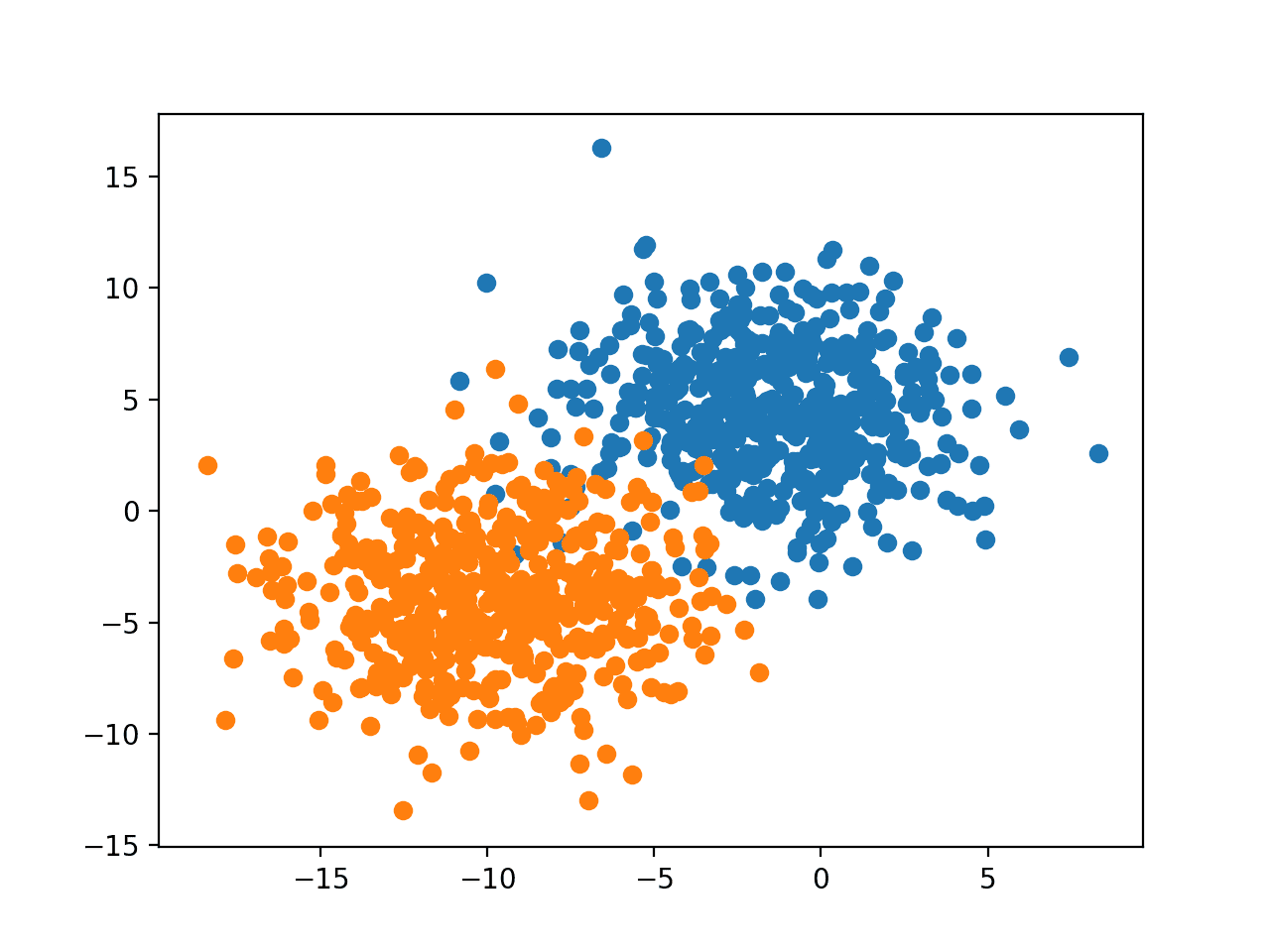
We can demonstrate this using a synthetic classification dataset with 1,000 examples.

The complete example is listed below.

# split a dataset into train and test sets
from sklearn.datasets import make_blobs
from sklearn.model_selection import train_test_split
# create dataset
X, y = make_blobs(n_samples=1000)
# split into train test sets
X_train, X_test, y_train, y_test = train_test_split(X, y, test_size=0.33)
print(X_train.shape, X_test.shape, y_train.shape, y_test.shape)

Running the example splits the dataset into train and test sets, then prints the size of the new dataset.

We can see that 670 examples (67 percent) were allocated to the training set and 330 examples (33 percent) were allocated to the test set, as we specified.

(670, 2) (330, 2) (670,) (330,)

Alternatively, the dataset can be split by specifying the “train_size” argument that can be either a number of rows (integer) or a percentage of the original dataset between 0 and 1, such as 0.67 for 67 percent.

...
# split into train test sets
X_train, X_test, y_train, y_test = train_test_split(X, y, train_size=0.67)

Repeatable Train-Test Splits

Another important consideration is that rows are assigned to the train and test sets randomly.

This is done to ensure that datasets are a representative sample (e.g. random sample) of the original dataset, which in turn, should be a representative sample of observations from the problem domain.

When comparing machine learning algorithms, it is desirable (perhaps required) that they are fit and evaluated on the same subsets of the dataset.

This can be achieved by fixing the seed for the pseudo-random number generator used when splitting the dataset. If you are new to pseudo-random number generators, see the tutorial:

This can be achieved by setting the “random_state” to an integer value. Any value will do; it is not a tunable hyperparameter.

...
# split again, and we should see the same split
X_train, X_test, y_train, y_test = train_test_split(X, y, test_size=0.33, random_state=1)

The example below demonstrates this and shows that two separate splits of the data result in the same result.

# demonstrate that the train-test split procedure is repeatable
from sklearn.datasets import make_blobs
from sklearn.model_selection import train_test_split
# create dataset
X, y = make_blobs(n_samples=100)
# split into train test sets
X_train, X_test, y_train, y_test = train_test_split(X, y, test_size=0.33, random_state=1)
# summarize first 5 rows
print(X_train[:5, :])
# split again, and we should see the same split
X_train, X_test, y_train, y_test = train_test_split(X, y, test_size=0.33, random_state=1)
# summarize first 5 rows
print(X_train[:5, :])

Running the example splits the dataset and prints the first five rows of the training dataset.

The dataset is split again and the first five rows of the training dataset are printed showing identical values, confirming that when we fix the seed for the pseudorandom number generator, we get an identical split of the original dataset.

[[-2.54341511  4.98947608]
 [ 5.65996724 -8.50997751]
 [-2.5072835  10.06155749]
 [ 6.92679558 -5.91095498]
 [ 6.01313957 -7.7749444 ]]

[[-2.54341511  4.98947608]
 [ 5.65996724 -8.50997751]
 [-2.5072835  10.06155749]
 [ 6.92679558 -5.91095498]
 [ 6.01313957 -7.7749444 ]]

Stratified Train-Test Splits

One final consideration is for classification problems only.

Some classification problems do not have a balanced number of examples for each class label. As such, it is desirable to split the dataset into train and test sets in a way that preserves the same proportions of examples in each class as observed in the original dataset.

This is called a stratified train-test split.

We can achieve this by setting the “stratify” argument to the y component of the original dataset. This will be used by the train_test_split() function to ensure that both the train and test sets have the proportion of examples in each class that is present in the provided “y” array.

...
# split into train test sets
X_train, X_test, y_train, y_test = train_test_split(X, y, test_size=0.50, random_state=1, stratify=y)

We can demonstrate this with an example of a classification dataset with 94 examples in one class and six examples in a second class.

First, we can split the dataset into train and test sets without the “stratify” argument. The complete example is listed below.

# split imbalanced dataset into train and test sets without stratification
from collections import Counter
from sklearn.datasets import make_classification
from sklearn.model_selection import train_test_split
# create dataset
X, y = make_classification(n_samples=100, weights=[0.94], flip_y=0, random_state=1)
print(Counter(y))
# split into train test sets
X_train, X_test, y_train, y_test = train_test_split(X, y, test_size=0.50, random_state=1)
print(Counter(y_train))
print(Counter(y_test))

Running the example first reports the composition of the dataset by class label, showing the expected 94 percent vs. 6 percent.

Then the dataset is split and the composition of the train and test sets is reported. We can see that the train set has 45/5 examples in the test set has 49/1 examples. The composition of the train and test sets differ, and this is not desirable.

Counter({0: 94, 1: 6})
Counter({0: 45, 1: 5})
Counter({0: 49, 1: 1})

Next, we can stratify the train-test split and compare the results.

# split imbalanced dataset into train and test sets with stratification
from collections import Counter
from sklearn.datasets import make_classification
from sklearn.model_selection import train_test_split
# create dataset
X, y = make_classification(n_samples=100, weights=[0.94], flip_y=0, random_state=1)
print(Counter(y))
# split into train test sets
X_train, X_test, y_train, y_test = train_test_split(X, y, test_size=0.50, random_state=1, stratify=y)
print(Counter(y_train))
print(Counter(y_test))

Given that we have used a 50 percent split for the train and test sets, we would expect both the train and test sets to have 47/3 examples in the train/test sets respectively.

Running the example, we can see that in this case, the stratified version of the train-test split has created both the train and test datasets with 47/3 examples in the train/test sets as we expected.

Counter({0: 94, 1: 6})
Counter({0: 47, 1: 3})

Now that we are familiar with the train_test_split() function, let’s look at how we can use it to evaluate a machine learning model.

Train-Test Split to Evaluate Machine Learning Models

In this section, we will explore using the train-test split procedure to evaluate machine learning models on standard classification and regression predictive modeling datasets.

Train-Test Split for Classification

We will demonstrate how to use the train-test split to evaluate a random forest algorithm on the sonar dataset.

The sonar dataset is a standard machine learning dataset composed of 208 rows of data with 60 numerical input variables and a target variable with two class values, e.g. binary classification.

The dataset involves predicting whether sonar returns indicate a rock or simulated mine.

No need to download the dataset; we will download it automatically as part of our worked examples.

The example below downloads the dataset and summarizes its shape.

# summarize the sonar dataset
from pandas import read_csv
# load dataset
url = 'https://raw.githubusercontent.com/jbrownlee/Datasets/master/sonar.csv'
dataframe = read_csv(url, header=None)
# split into input and output elements
data = dataframe.values
X, y = data[:, :-1], data[:, -1]
print(X.shape, y.shape)

Running the example downloads the dataset and splits it into input and output elements. As expected, we can see that there are 208 rows of data with 60 input variables.

(208, 60) (208,)

We can now evaluate a model using a train-test split.

First, the loaded dataset must be split into input and output components.

...
# split into inputs and outputs
X, y = data[:, :-1], data[:, -1]
print(X.shape, y.shape)

Next, we can split the dataset so that 67 percent is used to train the model and 33 percent is used to evaluate it. This split was chosen arbitrarily.

...
# split into train test sets
X_train, X_test, y_train, y_test = train_test_split(X, y, test_size=0.33, random_state=1)
print(X_train.shape, X_test.shape, y_train.shape, y_test.shape)

We can then define and fit the model on the training dataset.

...
# fit the model
model = RandomForestClassifier(random_state=1)
model.fit(X_train, y_train)

Then use the fit model to make predictions and evaluate the predictions using the classification accuracy performance metric.

...
# make predictions
yhat = model.predict(X_test)
# evaluate predictions
acc = accuracy_score(y_test, yhat)
print('Accuracy: %.3f' % acc)

Tying this together, the complete example is listed below.

# train-test split evaluation random forest on the sonar dataset
from pandas import read_csv
from sklearn.model_selection import train_test_split
from sklearn.ensemble import RandomForestClassifier
from sklearn.metrics import accuracy_score
# load dataset
url = 'https://raw.githubusercontent.com/jbrownlee/Datasets/master/sonar.csv'
dataframe = read_csv(url, header=None)
data = dataframe.values
# split into inputs and outputs
X, y = data[:, :-1], data[:, -1]
print(X.shape, y.shape)
# split into train test sets
X_train, X_test, y_train, y_test = train_test_split(X, y, test_size=0.33, random_state=1)
print(X_train.shape, X_test.shape, y_train.shape, y_test.shape)
# fit the model
model = RandomForestClassifier(random_state=1)
model.fit(X_train, y_train)
# make predictions
yhat = model.predict(X_test)
# evaluate predictions
acc = accuracy_score(y_test, yhat)
print('Accuracy: %.3f' % acc)

Running the example first loads the dataset and confirms the number of rows in the input and output elements.

The dataset is split into train and test sets and we can see that there are 139 rows for training and 69 rows for the test set.

Finally, the model is evaluated on the test set and the performance of the model when making predictions on new data has an accuracy of about 78.3 percent.

(208, 60) (208,)
(139, 60) (69, 60) (139,) (69,)
Accuracy: 0.783

Train-Test Split for Regression

We will demonstrate how to use the train-test split to evaluate a random forest algorithm on the housing dataset.

The housing dataset is a standard machine learning dataset composed of 506 rows of data with 13 numerical input variables and a numerical target variable.

The dataset involves predicting the house price given details of the house’s suburb in the American city of Boston.

No need to download the dataset; we will download it automatically as part of our worked examples.

The example below downloads and loads the dataset as a Pandas DataFrame and summarizes the shape of the dataset.

# load and summarize the housing dataset
from pandas import read_csv
# load dataset
url = 'https://raw.githubusercontent.com/jbrownlee/Datasets/master/housing.csv'
dataframe = read_csv(url, header=None)
# summarize shape
print(dataframe.shape)

Running the example confirms the 506 rows of data and 13 input variables and single numeric target variables (14 in total).

(506, 14)

We can now evaluate a model using a train-test split.

First, the loaded dataset must be split into input and output components.

...
# split into inputs and outputs
X, y = data[:, :-1], data[:, -1]
print(X.shape, y.shape)

Next, we can split the dataset so that 67 percent is used to train the model and 33 percent is used to evaluate it. This split was chosen arbitrarily.

...
# split into train test sets
X_train, X_test, y_train, y_test = train_test_split(X, y, test_size=0.33, random_state=1)
print(X_train.shape, X_test.shape, y_train.shape, y_test.shape)

We can then define and fit the model on the training dataset.

...
# fit the model
model = RandomForestRegressor(random_state=1)
model.fit(X_train, y_train)

Then use the fit model to make predictions and evaluate the predictions using the mean absolute error (MAE) performance metric.

...
# make predictions
yhat = model.predict(X_test)
# evaluate predictions
mae = mean_absolute_error(y_test, yhat)
print('MAE: %.3f' % mae)

Tying this together, the complete example is listed below.

# train-test split evaluation random forest on the housing dataset
from pandas import read_csv
from sklearn.model_selection import train_test_split
from sklearn.ensemble import RandomForestRegressor
from sklearn.metrics import mean_absolute_error
# load dataset
url = 'https://raw.githubusercontent.com/jbrownlee/Datasets/master/housing.csv'
dataframe = read_csv(url, header=None)
data = dataframe.values
# split into inputs and outputs
X, y = data[:, :-1], data[:, -1]
print(X.shape, y.shape)
# split into train test sets
X_train, X_test, y_train, y_test = train_test_split(X, y, test_size=0.33, random_state=1)
print(X_train.shape, X_test.shape, y_train.shape, y_test.shape)
# fit the model
model = RandomForestRegressor(random_state=1)
model.fit(X_train, y_train)
# make predictions
yhat = model.predict(X_test)
# evaluate predictions
mae = mean_absolute_error(y_test, yhat)
print('MAE: %.3f' % mae)

Running the example first loads the dataset and confirms the number of rows in the input and output elements.

The dataset is split into train and test sets and we can see that there are 339 rows for training and 167 rows for the test set.

Finally, the model is evaluated on the test set and the performance of the model when making predictions on new data is a mean absolute error of about 2.211 (thousands of dollars).

(506, 13) (506,)
(339, 13) (167, 13) (339,) (167,)
MAE: 2.157

Further Reading

This section provides more resources on the topic if you are looking to go deeper.

Summary

In this tutorial, you discovered how to evaluate machine learning models using the train-test split.

Specifically, you learned:

  • The train-test split procedure is appropriate when you have a very large dataset, a costly model to train, or require a good estimate of model performance quickly.
  • How to use the scikit-learn machine learning library to perform the train-test split procedure.
  • How to evaluate machine learning algorithms for classification and regression using the train-test split.

Do you have any questions?
Ask your questions in the comments below and I will do my best to answer.

The post Train-Test Split for Evaluating Machine Learning Algorithms appeared first on Machine Learning Mastery.


LOOCV for Evaluating Machine Learning Algorithms

$
0
0

The Leave-One-Out Cross-Validation, or LOOCV, procedure is used to estimate the performance of machine learning algorithms when they are used to make predictions on data not used to train the model.

It is a computationally expensive procedure to perform, although it results in a reliable and unbiased estimate of model performance. Although simple to use and no configuration to specify, there are times when the procedure should not be used, such as when you have a very large dataset or a computationally expensive model to evaluate.

In this tutorial, you will discover how to evaluate machine learning models using leave-one-out cross-validation.

After completing this tutorial, you will know:

  • The leave-one-out cross-validation procedure is appropriate when you have a small dataset or when an accurate estimate of model performance is more important than the computational cost of the method.
  • How to use the scikit-learn machine learning library to perform the leave-one-out cross-validation procedure.
  • How to evaluate machine learning algorithms for classification and regression using leave-one-out cross-validation.

Let’s get started.

LOOCV for Evaluating Machine Learning Algorithms

LOOCV for Evaluating Machine Learning Algorithms
Photo by Heather Harvey, some rights reserved.

Tutorial Overview

This tutorial is divided into three parts; they are:

  1. LOOCV Model Evaluation
  2. LOOCV Procedure in Scikit-Learn
  3. LOOCV to Evaluate Machine Learning Models
    1. LOOCV for Classification
    2. LOOCV for Regression

LOOCV Model Evaluation

Cross-validation, or k-fold cross-validation, is a procedure used to estimate the performance of a machine learning algorithm when making predictions on data not used during the training of the model.

The cross-validation has a single hyperparameter “k” that controls the number of subsets that a dataset is split into. Once split, each subset is given the opportunity to be used as a test set while all other subsets together are used as a training dataset.

This means that k-fold cross-validation involves fitting and evaluating k models. This, in turn, provides k estimates of a model’s performance on the dataset, which can be reported using summary statistics such as the mean and standard deviation. This score can then be used to compare and ultimately select a model and configuration to use as the “final model” for a dataset.

Typical values for k are k=3, k=5, and k=10, with 10 representing the most common value. This is because, given extensive testing, 10-fold cross-validation provides a good balance of low computational cost and low bias in the estimate of model performance as compared to other k values and a single train-test split.

For more on k-fold cross-validation, see the tutorial:

Leave-one-out cross-validation, or LOOCV, is a configuration of k-fold cross-validation where k is set to the number of examples in the dataset.

LOOCV is an extreme version of k-fold cross-validation that has the maximum computational cost. It requires one model to be created and evaluated for each example in the training dataset.

The benefit of so many fit and evaluated models is a more robust estimate of model performance as each row of data is given an opportunity to represent the entirety of the test dataset.

Given the computational cost, LOOCV is not appropriate for very large datasets such as more than tens or hundreds of thousands of examples, or for models that are costly to fit, such as neural networks.

  • Don’t Use LOOCV: Large datasets or costly models to fit.

Given the improved estimate of model performance, LOOCV is appropriate when an accurate estimate of model performance is critical. This particularly case when the dataset is small, such as less than thousands of examples, can lead to model overfitting during training and biased estimates of model performance.

Further, given that no sampling of the training dataset is used, this estimation procedure is deterministic, unlike train-test splits and other k-fold cross-validation confirmations that provide a stochastic estimate of model performance.

  • Use LOOCV: Small datasets or when estimated model performance is critical.

Once models have been evaluated using LOOCV and a final model and configuration chosen, a final model is then fit on all available data and used to make predictions on new data.

Now that we are familiar with the LOOCV procedure, let’s look at how we can use the method in Python.

LOOCV Procedure in Scikit-Learn

The scikit-learn Python machine learning library provides an implementation of the LOOCV via the LeaveOneOut class.

The method has no configuration, therefore, no arguments are provided to create an instance of the class.

...
# create loocv procedure
cv = LeaveOneOut()

Once created, the split() function can be called and provided the dataset to enumerate.

Each iteration will return the row indices that can be used for the train and test sets from the provided dataset.

...
for train_ix, test_ix in cv.split(X):
	...

These indices can be used on the input (X) and output (y) columns of the dataset array to split the dataset.

...
# split data
X_train, X_test = X[train_ix, :], X[test_ix, :]
y_train, y_test = y[train_ix], y[test_ix]

The training set can be used to fit a model and the test set can be used to evaluate it by first making a prediction and calculating a performance metric on the predicted values versus the expected values.

...
# fit model
model = RandomForestClassifier(random_state=1)
model.fit(X_train, y_train)
# evaluate model
yhat = model.predict(X_test)

Scores can be saved from each evaluation and a final mean estimate of model performance can be presented.

We can tie this together and demonstrate how to use LOOCV to evaluate a RandomForestClassifier model for a synthetic binary classification dataset created with the make_blobs() function.

The complete example is listed below.

# loocv to manually evaluate the performance of a random forest classifier
from sklearn.datasets import make_blobs
from sklearn.model_selection import LeaveOneOut
from sklearn.ensemble import RandomForestClassifier
from sklearn.metrics import accuracy_score
# create dataset
X, y = make_blobs(n_samples=100, random_state=1)
# create loocv procedure
cv = LeaveOneOut()
# enumerate splits
y_true, y_pred = list(), list()
for train_ix, test_ix in cv.split(X):
	# split data
	X_train, X_test = X[train_ix, :], X[test_ix, :]
	y_train, y_test = y[train_ix], y[test_ix]
	# fit model
	model = RandomForestClassifier(random_state=1)
	model.fit(X_train, y_train)
	# evaluate model
	yhat = model.predict(X_test)
	# store
	y_true.append(y_test[0])
	y_pred.append(yhat[0])
# calculate accuracy
acc = accuracy_score(y_true, y_pred)
print('Accuracy: %.3f' % acc)

Running the example manually estimates the performance of the random forest classifier on the synthetic dataset.

Given that the dataset has 100 examples, it means that 100 train/test splits of the dataset were created, with each single row of the dataset given an opportunity to be used as the test set. Similarly, 100 models are created and evaluated.

The classification accuracy across all predictions is then reported, in this case as 99 percent.

Accuracy: 0.990

A downside of enumerating the folds manually is that it is slow and involves a lot of code that could introduce bugs.

An alternative to evaluating a model using LOOCV is to use the cross_val_score() function.

This function takes the model, the dataset, and the instantiated LOOCV object set via the “cv” argument. A sample of accuracy scores is then returned that can be summarized by calculating the mean and standard deviation.

We can also set the “n_jobs” argument to -1 to use all CPU cores, greatly decreasing the computational cost in fitting and evaluating so many models.

The example below demonstrates evaluating the RandomForestClassifier using LOOCV on the same synthetic dataset using the cross_val_score() function.

# loocv to automatically evaluate the performance of a random forest classifier
from numpy import mean
from numpy import std
from sklearn.datasets import make_blobs
from sklearn.model_selection import LeaveOneOut
from sklearn.model_selection import cross_val_score
from sklearn.ensemble import RandomForestClassifier
# create dataset
X, y = make_blobs(n_samples=100, random_state=1)
# create loocv procedure
cv = LeaveOneOut()
# create model
model = RandomForestClassifier(random_state=1)
# evaluate model
scores = cross_val_score(model, X, y, scoring='accuracy', cv=cv, n_jobs=-1)
# report performance
print('Accuracy: %.3f (%.3f)' % (mean(scores), std(scores)))

Running the example automatically estimates the performance of the random forest classifier on the synthetic dataset.

The mean classification accuracy across all folds matches our manual estimate previously.

Accuracy: 0.990 (0.099)

Now that we are familiar with how to use the LeaveOneOut class, let’s look at how we can use it to evaluate a machine learning model on real datasets.

LOOCV to Evaluate Machine Learning Models

In this section, we will explore using the LOOCV procedure to evaluate machine learning models on standard classification and regression predictive modeling datasets.

LOOCV for Classification

We will demonstrate how to use LOOCV to evaluate a random forest algorithm on the sonar dataset.

The sonar dataset is a standard machine learning dataset comprising 208 rows of data with 60 numerical input variables and a target variable with two class values, e.g. binary classification.

The dataset involves predicting whether sonar returns indicate a rock or simulated mine.

No need to download the dataset; we will download it automatically as part of our worked examples.

The example below downloads the dataset and summarizes its shape.

# summarize the sonar dataset
from pandas import read_csv
# load dataset
url = 'https://raw.githubusercontent.com/jbrownlee/Datasets/master/sonar.csv'
dataframe = read_csv(url, header=None)
# split into input and output elements
data = dataframe.values
X, y = data[:, :-1], data[:, -1]
print(X.shape, y.shape)

Running the example downloads the dataset and splits it into input and output elements. As expected, we can see that there are 208 rows of data with 60 input variables.

(208, 60) (208,)

We can now evaluate a model using LOOCV.

First, the loaded dataset must be split into input and output components.

...
# split into inputs and outputs
X, y = data[:, :-1], data[:, -1]
print(X.shape, y.shape)

Next, we define the LOOCV procedure.

...
# create loocv procedure
cv = LeaveOneOut()

We can then define the model to evaluate.

...
# create model
model = RandomForestClassifier(random_state=1)

Then use the cross_val_score() function to enumerate the folds, fit models, then make and evaluate predictions. We can then report the mean and standard deviation of model performance.

...
# evaluate model
scores = cross_val_score(model, X, y, scoring='accuracy', cv=cv, n_jobs=-1)
# report performance
print('Accuracy: %.3f (%.3f)' % (mean(scores), std(scores)))

Tying this together, the complete example is listed below.

# loocv evaluate random forest on the sonar dataset
from numpy import mean
from numpy import std
from pandas import read_csv
from sklearn.model_selection import LeaveOneOut
from sklearn.model_selection import cross_val_score
from sklearn.ensemble import RandomForestClassifier
# load dataset
url = 'https://raw.githubusercontent.com/jbrownlee/Datasets/master/sonar.csv'
dataframe = read_csv(url, header=None)
data = dataframe.values
# split into inputs and outputs
X, y = data[:, :-1], data[:, -1]
print(X.shape, y.shape)
# create loocv procedure
cv = LeaveOneOut()
# create model
model = RandomForestClassifier(random_state=1)
# evaluate model
scores = cross_val_score(model, X, y, scoring='accuracy', cv=cv, n_jobs=-1)
# report performance
print('Accuracy: %.3f (%.3f)' % (mean(scores), std(scores)))

Running the example first loads the dataset and confirms the number of rows in the input and output elements.

The model is then evaluated using LOOCV and the estimated performance when making predictions on new data has an accuracy of about 82.2 percent.

(208, 60) (208,)
Accuracy: 0.822 (0.382)

LOOCV for Regression

We will demonstrate how to use LOOCV to evaluate a random forest algorithm on the housing dataset.

The housing dataset is a standard machine learning dataset comprising 506 rows of data with 13 numerical input variables and a numerical target variable.

The dataset involves predicting the house price given details of the house’s suburb in the American city of Boston.

No need to download the dataset; we will download it automatically as part of our worked examples.

The example below downloads and loads the dataset as a Pandas DataFrame and summarizes the shape of the dataset.

# load and summarize the housing dataset
from pandas import read_csv
# load dataset
url = 'https://raw.githubusercontent.com/jbrownlee/Datasets/master/housing.csv'
dataframe = read_csv(url, header=None)
# summarize shape
print(dataframe.shape)

Running the example confirms the 506 rows of data and 13 input variables and single numeric target variables (14 in total).

(506, 14)

We can now evaluate a model using LOOCV.

First, the loaded dataset must be split into input and output components.

...
# split into inputs and outputs
X, y = data[:, :-1], data[:, -1]
print(X.shape, y.shape)

Next, we define the LOOCV procedure.

...
# create loocv procedure
cv = LeaveOneOut()

We can then define the model to evaluate.

...
# create model
model = RandomForestRegressor(random_state=1)

Then use the cross_val_score() function to enumerate the folds, fit models, then make and evaluate predictions. We can then report the mean and standard deviation of model performance.

In this case, we use the mean absolute error (MAE) performance metric appropriate for regression.

...
# evaluate model
scores = cross_val_score(model, X, y, scoring='neg_mean_absolute_error', cv=cv, n_jobs=-1)
# force positive
scores = absolute(scores)
# report performance
print('MAE: %.3f (%.3f)' % (mean(scores), std(scores)))

Tying this together, the complete example is listed below.

# loocv evaluate random forest on the housing dataset
from numpy import mean
from numpy import std
from numpy import absolute
from pandas import read_csv
from sklearn.model_selection import LeaveOneOut
from sklearn.model_selection import cross_val_score
from sklearn.ensemble import RandomForestRegressor
# load dataset
url = 'https://raw.githubusercontent.com/jbrownlee/Datasets/master/housing.csv'
dataframe = read_csv(url, header=None)
data = dataframe.values
# split into inputs and outputs
X, y = data[:, :-1], data[:, -1]
print(X.shape, y.shape)
# create loocv procedure
cv = LeaveOneOut()
# create model
model = RandomForestRegressor(random_state=1)
# evaluate model
scores = cross_val_score(model, X, y, scoring='neg_mean_absolute_error', cv=cv, n_jobs=-1)
# force positive
scores = absolute(scores)
# report performance
print('MAE: %.3f (%.3f)' % (mean(scores), std(scores)))

Running the example first loads the dataset and confirms the number of rows in the input and output elements.

The model is evaluated using LOOCV and the performance of the model when making predictions on new data is a mean absolute error of about 2.180 (thousands of dollars).

(506, 13) (506,)
MAE: 2.180 (2.346)

Further Reading

This section provides more resources on the topic if you are looking to go deeper.

Tutorials

APIs

Summary

In this tutorial, you discovered how to evaluate machine learning models using leave-one-out cross-validation.

Specifically, you learned:

  • The leave-one-out cross-validation procedure is appropriate when you have a small dataset or when an accurate estimate of model performance is more important than the computational cost of the method.
  • How to use the scikit-learn machine learning library to perform the leave-one-out cross-validation procedure.
  • How to evaluate machine learning algorithms for classification and regression using leave-one-out cross-validation.

Do you have any questions?
Ask your questions in the comments below and I will do my best to answer.

The post LOOCV for Evaluating Machine Learning Algorithms appeared first on Machine Learning Mastery.

Nested Cross-Validation for Machine Learning with Python

$
0
0

The k-fold cross-validation procedure is used to estimate the performance of machine learning models when making predictions on data not used during training.

This procedure can be used both when optimizing the hyperparameters of a model on a dataset, and when comparing and selecting a model for the dataset. When the same cross-validation procedure and dataset are used to both tune and select a model, it is likely to lead to an optimistically biased evaluation of the model performance.

One approach to overcoming this bias is to nest the hyperparameter optimization procedure under the model selection procedure. This is called double cross-validation or nested cross-validation and is the preferred way to evaluate and compare tuned machine learning models.

In this tutorial, you will discover nested cross-validation for evaluating tuned machine learning models.

After completing this tutorial, you will know:

  • Hyperparameter optimization can overfit a dataset and provide an optimistic evaluation of a model that should not be used for model selection.
  • Nested cross-validation provides a way to reduce the bias in combined hyperparameter tuning and model selection.
  • How to implement nested cross-validation for evaluating tuned machine learning algorithms in scikit-learn.

Let’s get started.

Nested Cross-Validation for Machine Learning with Python

Nested Cross-Validation for Machine Learning with Python
Photo by Andrew Bone, some rights reserved.

Tutorial Overview

This tutorial is divided into three parts; they are:

  1. Combined Hyperparameter Tuning and Model Selection
  2. What Is Nested Cross-Validation
  3. Nested Cross-Validation With Scikit-Learn

Combined Hyperparameter Tuning and Model Selection

It is common to evaluate machine learning models on a dataset using k-fold cross-validation.

The k-fold cross-validation procedure divides a limited dataset into k non-overlapping folds. Each of the k folds is given an opportunity to be used as a held back test set whilst all other folds collectively are used as a training dataset. A total of k models are fit and evaluated on the k holdout test sets and the mean performance is reported.

For more on the k-fold cross-validation procedure, see the tutorial:

The procedure provides an estimate of the model performance on the dataset when making a prediction on data not used during training. It is less biased than some other techniques, such as a single train-test split for small- to modestly-sized dataset. Common values for k are k=3, k=5, and k=10.

Each machine learning algorithm includes one or more hyperparameters that allow the algorithm behavior to be tailored to a specific dataset. The trouble is, there is rarely if ever good heuristics on how to configure the model hyperparameters for a dataset. Instead, an optimization procedure is used to discover a set of hyperparameters that perform well or best on the dataset. Common examples of optimization algorithms include grid search and random search, and each distinct set of model hyperparameters are typically evaluated using k-fold cross-validation.

This highlights that the k-fold cross-validation procedure is used both in the selection of model hyperparameters to configure each model and in the selection of configured models.

The k-fold cross-validation procedure is an effective approach for estimating the performance of a model. Nevertheless, a limitation of the procedure is that if it is used multiple times with the same algorithm, it can lead to overfitting.

Each time a model with different model hyperparameters is evaluated on a dataset, it provides information about the dataset. Specifically, an often noisy model performance score. This knowledge about the model on the dataset can be exploited in the model configuration procedure to find the best performing configuration for the dataset. The k-fold cross-validation procedure attempts to reduce this effect, yet it cannot be removed completely, and some form of hill-climbing or overfitting of the model hyperparameters to the dataset will be performed. This is the normal case for hyperparameter optimization.

The problem is that if this score alone is used to then select a model, or the same dataset is used to evaluate the tuned models, then the selection process will be biased by this inadvertent overfitting. The result is an overly optimistic estimate of model performance that does not generalize to new data.

A procedure is required that allows both the models to select well-performing hyperparameters for the dataset and select among a collection of well-configured models on a dataset.

One approach to this problem is called nested cross-validation.

What Is Nested Cross-Validation

Nested cross-validation is an approach to model hyperparameter optimization and model selection that attempts to overcome the problem of overfitting the training dataset.

In order to overcome the bias in performance evaluation, model selection should be viewed as an integral part of the model fitting procedure, and should be conducted independently in each trial in order to prevent selection bias and because it reflects best practice in operational use.

On Over-fitting in Model Selection and Subsequent Selection Bias in Performance Evaluation, 2010.

The procedure involves treating model hyperparameter optimization as part of the model itself and evaluating it within the broader k-fold cross-validation procedure for evaluating models for comparison and selection.

As such, the k-fold cross-validation procedure for model hyperparameter optimization is nested inside the k-fold cross-validation procedure for model selection. The use of two cross-validation loops also leads the procedure to be called “double cross-validation.”

Typically, the k-fold cross-validation procedure involves fitting a model on all folds but one and evaluating the fit model on the holdout fold. Let’s refer to the aggregate of folds used to train the model as the “train dataset” and the held-out fold as the “test dataset.”

Each training dataset is then provided to a hyperparameter optimized procedure, such as grid search or random search, that finds an optimal set of hyperparameters for the model. The evaluation of each set of hyperparameters is performed using k-fold cross-validation that splits up the provided train dataset into k folds, not the original dataset.

This is termed the “internal” protocol as the model selection process is performed independently within each fold of the resampling procedure.

On Over-fitting in Model Selection and Subsequent Selection Bias in Performance Evaluation, 2010.

Under this procedure, hyperparameter search does not have an opportunity to overfit the dataset as it is only exposed to a subset of the dataset provided by the outer cross-validation procedure. This reduces, if not eliminates, the risk of the search procedure overfitting the original dataset and should provide a less biased estimate of a tuned model’s performance on the dataset.

In this way, the performance estimate includes a component properly accounting for the error introduced by overfitting the model selection criterion.

On Over-fitting in Model Selection and Subsequent Selection Bias in Performance Evaluation, 2010.

What Is the Cost of Nested Cross-Validation?

A downside of nested cross-validation is the dramatic increase in the number of model evaluations performed.

If n * k models are fit and evaluated as part of a traditional cross-validation hyperparameter search for a given model, then this is increased to k * n * k as the procedure is then performed k more times for each fold in the outer loop of nested cross-validation.

To make this concrete, you might use k=5 for the hyperparameter search and test 100 combinations of model hyperparameters. A traditional hyperparameter search would, therefore, fit and evaluate 5 * 100 or 500 models. Nested cross-validation with k=10 folds in the outer loop would fit and evaluate 5,000 models. A 10x increase in this case.

How Do You Set k?

The k value for the inner loop and the outer loop should be set as you would set the k-value for a single k-fold cross-validation procedure.

You must choose a k-value for your dataset that balances the computational cost of the evaluation procedure (not too many model evaluations) and unbiased estimate of model performance.

It is common to use k=10 for the outer loop and a smaller value of k for the inner loop, such as k=3 or k=5.

How Do You Configure the Final Model?

The final model is configured and fit using the procedure applied internally to the outer loop.

As follows:

  1. An algorithm is selected based on its performance on the outer loop of nested cross-validation.
  2. Then the inner-procedure is applied to the entire dataset.
  3. The hyperparameters found during this final search are then used to configure a final model.
  4. The final model is fit on the entire dataset.

This model can then be used to make predictions on new data. We know how well it will perform on average based on the score provided during the final model tuning procedure.

Now that we are familiar with nested-cross validation, let’s review how we can implement it in practice.

Nested Cross-Validation With Scikit-Learn

The k-fold cross-validation procedure is available in the scikit-learn Python machine learning library via the KFold class.

The class is configured with the number of folds (splits), then the split() function is called, passing in the dataset. The results of the split() function are enumerated to give the row indexes for the train and test sets for each fold.

For example:

...
# configure the cross-validation procedure
cv = KFold(n_splits=10, random_state=1)
# perform cross-validation procedure
for train_ix, test_ix in cv_outer.split(X):
	# split data
	X_train, X_test = X[train_ix, :], X[test_ix, :]
	y_train, y_test = y[train_ix], y[test_ix]
	# fit and evaluate a model
	...

This class can be used to perform the outer-loop of the nested-cross validation procedure.

The scikit-learn library provides cross-validation random search and grid search hyperparameter optimization via the RandomizedSearchCV and GridSearchCV classes respectively. The procedure is configured by creating the class and specifying the model, dataset, hyperparameters to search, and cross-validation procedure.

For example:

...
# configure the cross-validation procedure
cv = KFold(n_splits=3, shuffle=True, random_state=1)
# define search space
space = dict()
...
# define search
search = GridSearchCV(model, space, scoring='accuracy', n_jobs=-1, cv=cv)
# execute search
result = search.fit(X, y)

These classes can be used for the inner loop of nested cross-validation where the train dataset defined by the outer loop is used as the dataset for the inner loop.

We can tie these elements together and implement the nested cross-validation procedure.

Importantly, we can configure the hyperparameter search to refit a final model with the entire training dataset using the best hyperparameters found during the search. This can be achieved by setting the “refit” argument to True, then retrieving the model via the “best_estimator_” attribute on the search result.

...
# define search
search = GridSearchCV(model, space, scoring='accuracy', n_jobs=-1, cv=cv_inner, refit=True)
# execute search
result = search.fit(X_train, y_train)
# get the best performing model fit on the whole training set
best_model = result.best_estimator_

This model can then be used to make predictions on the holdout data from the outer loop and estimate the performance of the model.

...
# evaluate model on the hold out dataset
yhat = best_model.predict(X_test)

Tying all of this together, we can demonstrate nested cross-validation for the RandomForestClassifier on a synthetic classification dataset.

We will keep things simple and tune just two hyperparameters with three values each, e.g. (3 * 3) 9 combinations. We will use 10 folds in the outer cross-validation and three folds for the inner cross-validation, resulting in (10 * 9 * 3) or 270 model evaluations.

The complete example is listed below.

# manual nested cross-validation for random forest on a classification dataset
from numpy import mean
from numpy import std
from sklearn.datasets import make_classification
from sklearn.model_selection import KFold
from sklearn.model_selection import GridSearchCV
from sklearn.ensemble import RandomForestClassifier
from sklearn.metrics import accuracy_score
# create dataset
X, y = make_classification(n_samples=1000, n_features=20, random_state=1, n_informative=10, n_redundant=10)
# configure the cross-validation procedure
cv_outer = KFold(n_splits=10, shuffle=True, random_state=1)
# enumerate splits
outer_results = list()
for train_ix, test_ix in cv_outer.split(X):
	# split data
	X_train, X_test = X[train_ix, :], X[test_ix, :]
	y_train, y_test = y[train_ix], y[test_ix]
	# configure the cross-validation procedure
	cv_inner = KFold(n_splits=3, shuffle=True, random_state=1)
	# define the model
	model = RandomForestClassifier(random_state=1)
	# define search space
	space = dict()
	space['n_estimators'] = [10, 100, 500]
	space['max_features'] = [2, 4, 6]
	# define search
	search = GridSearchCV(model, space, scoring='accuracy', cv=cv_inner, refit=True)
	# execute search
	result = search.fit(X_train, y_train)
	# get the best performing model fit on the whole training set
	best_model = result.best_estimator_
	# evaluate model on the hold out dataset
	yhat = best_model.predict(X_test)
	# evaluate the model
	acc = accuracy_score(y_test, yhat)
	# store the result
	outer_results.append(acc)
	# report progress
	print('>acc=%.3f, est=%.3f, cfg=%s' % (acc, result.best_score_, result.best_params_))
# summarize the estimated performance of the model
print('Accuracy: %.3f (%.3f)' % (mean(outer_results), std(outer_results)))

Running the example evaluates random forest using nested-cross validation on a synthetic classification dataset.

You can use the example as a starting point and adapt it to evaluate different algorithm hyperparameters, different algorithms, or a different dataset.

Each iteration of the outer cross-validation procedure reports the estimated performance of the best performing model (using 3-fold cross-validation) and the hyperparameters found to perform the best, as well as the accuracy on the holdout dataset.

This is insightful as we can see that the actual and estimated accuracies are different, but in this case, similar. We can also see that different hyperparameters are found on each iteration, showing that good hyperparameters on this dataset are dependent on the specifics of the dataset.

A final mean classification accuracy is then reported.

>acc=0.900, est=0.932, cfg={'max_features': 4, 'n_estimators': 100}
>acc=0.940, est=0.924, cfg={'max_features': 4, 'n_estimators': 500}
>acc=0.930, est=0.929, cfg={'max_features': 4, 'n_estimators': 500}
>acc=0.930, est=0.927, cfg={'max_features': 6, 'n_estimators': 100}
>acc=0.920, est=0.927, cfg={'max_features': 4, 'n_estimators': 100}
>acc=0.950, est=0.927, cfg={'max_features': 4, 'n_estimators': 500}
>acc=0.910, est=0.918, cfg={'max_features': 2, 'n_estimators': 100}
>acc=0.930, est=0.924, cfg={'max_features': 6, 'n_estimators': 500}
>acc=0.960, est=0.926, cfg={'max_features': 2, 'n_estimators': 500}
>acc=0.900, est=0.937, cfg={'max_features': 4, 'n_estimators': 500}
Accuracy: 0.927 (0.019)

A simpler way that we can perform the same procedure is by using the cross_val_score() function that will execute the outer cross-validation procedure. This can be performed on the configured GridSearchCV directly that will automatically use the refit best performing model on the test set from the outer loop.

This greatly reduces the amount of code required to perform the nested cross-validation.

The complete example is listed below.

# automatic nested cross-validation for random forest on a classification dataset
from numpy import mean
from numpy import std
from sklearn.datasets import make_classification
from sklearn.model_selection import cross_val_score
from sklearn.model_selection import KFold
from sklearn.model_selection import GridSearchCV
from sklearn.ensemble import RandomForestClassifier
# create dataset
X, y = make_classification(n_samples=1000, n_features=20, random_state=1, n_informative=10, n_redundant=10)
# configure the cross-validation procedure
cv_inner = KFold(n_splits=3, shuffle=True, random_state=1)
# define the model
model = RandomForestClassifier(random_state=1)
# define search space
space = dict()
space['n_estimators'] = [10, 100, 500]
space['max_features'] = [2, 4, 6]
# define search
search = GridSearchCV(model, space, scoring='accuracy', n_jobs=1, cv=cv_inner, refit=True)
# configure the cross-validation procedure
cv_outer = KFold(n_splits=10, shuffle=True, random_state=1)
# execute the nested cross-validation
scores = cross_val_score(search, X, y, scoring='accuracy', cv=cv_outer, n_jobs=-1)
# report performance
print('Accuracy: %.3f (%.3f)' % (mean(scores), std(scores)))

Running the examples performs the nested cross-validation on the random forest algorithm, achieving a mean accuracy that matches our manual procedure.

Accuracy: 0.927 (0.019)

Further Reading

This section provides more resources on the topic if you are looking to go deeper.

Tutorials

Papers

APIs

Summary

In this tutorial, you discovered nested cross-validation for evaluating tuned machine learning models.

Specifically, you learned:

  • Hyperparameter optimization can overfit a dataset and provide an optimistic evaluation of a model that should not be used for model selection.
  • Nested cross-validation provides a way to reduce the bias in combined hyperparameter tuning and model selection.
  • How to implement nested cross-validation for evaluating tuned machine learning algorithms in scikit-learn.

Do you have any questions?
Ask your questions in the comments below and I will do my best to answer.

The post Nested Cross-Validation for Machine Learning with Python appeared first on Machine Learning Mastery.

How to Configure k-Fold Cross-Validation

$
0
0

The k-fold cross-validation procedure is a standard method for estimating the performance of a machine learning algorithm on a dataset.

A common value for k is 10, although how do we know that this configuration is appropriate for our dataset and our algorithms?

One approach is to explore the effect of different k values on the estimate of model performance and compare this to an ideal test condition. This can help to choose an appropriate value for k.

Once a k-value is chosen, it can be used to evaluate a suite of different algorithms on the dataset and the distribution of results can be compared to an evaluation of the same algorithms using an ideal test condition to see if they are highly correlated or not. If correlated, it confirms the chosen configuration is a robust approximation for the ideal test condition.

In this tutorial, you will discover how to configure and evaluate configurations of k-fold cross-validation.

After completing this tutorial, you will know:

  • How to evaluate a machine learning algorithm using k-fold cross-validation on a dataset.
  • How to perform a sensitivity analysis of k-values for k-fold cross-validation.
  • How to calculate the correlation between a cross-validation test harness and an ideal test condition.

Let’s get started.

How to Configure k-Fold Cross-Validation

How to Configure k-Fold Cross-Validation
Photo by Patricia Farrell, some rights reserved.

Tutorial Overview

This tutorial is divided into three parts; they are:

  1. k-Fold Cross-Validation
  2. Sensitivity Analysis for k
  3. Correlation of Test Harness With Target

k-Fold Cross-Validation

It is common to evaluate machine learning models on a dataset using k-fold cross-validation.

The k-fold cross-validation procedure divides a limited dataset into k non-overlapping folds. Each of the k folds is given an opportunity to be used as a held-back test set, whilst all other folds collectively are used as a training dataset. A total of k models are fit and evaluated on the k hold-out test sets and the mean performance is reported.

For more on the k-fold cross-validation procedure, see the tutorial:

The k-fold cross-validation procedure can be implemented easily using the scikit-learn machine learning library.

First, let’s define a synthetic classification dataset that we can use as the basis of this tutorial.

The make_classification() function can be used to create a synthetic binary classification dataset. We will configure it to generate 100 samples each with 20 input features, 15 of which contribute to the target variable.

The example below creates and summarizes the dataset.

# test classification dataset
from sklearn.datasets import make_classification
# define dataset
X, y = make_classification(n_samples=100, n_features=20, n_informative=15, n_redundant=5, random_state=1)
# summarize the dataset
print(X.shape, y.shape)

Running the example creates the dataset and confirms that it contains 100 samples and 10 input variables.

The fixed seed for the pseudorandom number generator ensures that we get the same samples each time the dataset is generated.

(100, 20) (100,)

Next, we can evaluate a model on this dataset using k-fold cross-validation.

We will evaluate a LogisticRegression model and use the KFold class to perform the cross-validation, configured to shuffle the dataset and set k=10, a popular default.

The cross_val_score() function will be used to perform the evaluation, taking the dataset and cross-validation configuration and returning a list of scores calculated for each fold.

The complete example is listed below.

# evaluate a logistic regression model using k-fold cross-validation
from numpy import mean
from numpy import std
from sklearn.datasets import make_classification
from sklearn.model_selection import KFold
from sklearn.model_selection import cross_val_score
from sklearn.linear_model import LogisticRegression
# create dataset
X, y = make_classification(n_samples=100, n_features=20, n_informative=15, n_redundant=5, random_state=1)
# prepare the cross-validation procedure
cv = KFold(n_splits=10, random_state=1, shuffle=True)
# create model
model = LogisticRegression()
# evaluate model
scores = cross_val_score(model, X, y, scoring='accuracy', cv=cv, n_jobs=-1)
# report performance
print('Accuracy: %.3f (%.3f)' % (mean(scores), std(scores)))

Running the example creates the dataset, then evaluates a logistic regression model on it using 10-fold cross-validation. The mean classification accuracy on the dataset is then reported.

Your specific results may vary given the stochastic nature of the learning algorithm. Try running the example a few times.

In this case, we can see that the model achieved an estimated classification accuracy of about 85.0 percent.

Accuracy: 0.850 (0.128)

Now that we are familiar with k-fold cross-validation, let’s look at how we might configure the procedure.

Sensitivity Analysis for k

The key configuration parameter for k-fold cross-validation is k that defines the number folds in which to split a given dataset.

Common values are k=3, k=5, and k=10, and by far the most popular value used in applied machine learning to evaluate models is k=10. The reason for this is studies were performed and k=10 was found to provide good trade-off of low computational cost and low bias in an estimate of model performance.

How do we know what value of k to use when evaluating models on our own dataset?

You can choose k=10, but how do you know this makes sense for your dataset?

One approach to answering this question is to perform a sensitivity analysis for different k values. That is, evaluate the performance of the same model on the same dataset with different values of k and see how they compare.

The expectation is that low values of k will result in a noisy estimate of model performance and large values of k will result in a less noisy estimate of model performance.

But noisy compared to what?

We don’t know the true performance of the model when making predictions on new/unseen data, as we don’t have access to new/unseen data. If we did, we would make use of it in the evaluation of the model.

Nevertheless, we can choose a test condition that represents an “ideal” or as-best-as-we-can-achieve “ideal” estimate of model performance.

One approach would be to train the model on all available data and estimate the performance on a separate large and representative hold-out dataset. The performance on this hold-out dataset would represent the “true” performance of the model and any cross-validation performances on the training dataset would represent an estimate of this score.

This is rarely possible as we often do not have enough data to hold some back and use it as a test set. Kaggle machine learning competitions are one exception to this, where we do have a hold-out test set, a sample of which is evaluated via submissions.

Instead, we can simulate this case using the leave-one-out cross-validation (LOOCV), a computationally expensive version of cross-validation where k=N, and N is the total number of examples in the training dataset. That is, each sample in the training set is given an example to be used alone as the test evaluation dataset. It is rarely used for large datasets as it is computationally expensive, although it can provide a good estimate of model performance given the available data.

We can then compare the mean classification accuracy for different k values to the mean classification accuracy from LOOCV on the same dataset. The difference between the scores provides a rough proxy for how well a k value approximates the ideal model evaluation test condition.

Let’s explore how to implement a sensitivity analysis of k-fold cross-validation.

First, let’s define a function to create the dataset. This allows you to change the dataset to your own if you desire.

# create the dataset
def get_dataset(n_samples=100):
	X, y = make_classification(n_samples=n_samples, n_features=20, n_informative=15, n_redundant=5, random_state=1)
	return X, y

Next, we can define a dataset to create the model to evaluate.

Again, this separation allows you to change the model to your own if you desire.

# retrieve the model to be evaluate
def get_model():
	model = LogisticRegression()
	return model

Next, you can define a function to evaluate the model on the dataset given a test condition. The test condition could be an instance of the KFold configured with a given k-value, or it could be an instance of LeaveOneOut that represents our ideal test condition.

The function returns the mean classification accuracy as well as the min and max accuracy from the folds. We can use the min and max to summarize the distribution of scores.

# evaluate the model using a given test condition
def evaluate_model(cv):
	# get the dataset
	X, y = get_dataset()
	# get the model
	model = get_model()
	# evaluate the model
	scores = cross_val_score(model, X, y, scoring='accuracy', cv=cv, n_jobs=-1)
	# return scores
	return mean(scores), scores.min(), scores.max()

Next, we can calculate the model performance using the LOOCV procedure.

...
# calculate the ideal test condition
ideal, _, _ = evaluate_model(LeaveOneOut())
print('Ideal: %.3f' % ideal)

We can then define the k values to evaluate. In this case, we will test values between 2 and 30.

...
# define folds to test
folds = range(2,31)

We can then evaluate each value in turn and store the results as we go.

...
# record mean and min/max of each set of results
means, mins, maxs = list(),list(),list()
# evaluate each k value
for k in folds:
	# define the test condition
	cv = KFold(n_splits=k, shuffle=True, random_state=1)
	# evaluate k value
	k_mean, k_min, k_max = evaluate_model(cv)
	# report performance
	print('> folds=%d, accuracy=%.3f (%.3f,%.3f)' % (k, k_mean, k_min, k_max))
	# store mean accuracy
	means.append(k_mean)
	# store min and max relative to the mean
	mins.append(k_mean - k_min)
	maxs.append(k_max - k_mean)

Finally, we can plot the results for interpretation.

...
# line plot of k mean values with min/max error bars
pyplot.errorbar(folds, means, yerr=[mins, maxs], fmt='o')
# plot the ideal case in a separate color
pyplot.plot(folds, [ideal for _ in range(len(folds))], color='r')
# show the plot
pyplot.show()

Tying this together, the complete example is listed below.

# sensitivity analysis of k in k-fold cross-validation
from numpy import mean
from sklearn.datasets import make_classification
from sklearn.model_selection import LeaveOneOut
from sklearn.model_selection import KFold
from sklearn.model_selection import cross_val_score
from sklearn.linear_model import LogisticRegression
from matplotlib import pyplot

# create the dataset
def get_dataset(n_samples=100):
	X, y = make_classification(n_samples=n_samples, n_features=20, n_informative=15, n_redundant=5, random_state=1)
	return X, y

# retrieve the model to be evaluate
def get_model():
	model = LogisticRegression()
	return model

# evaluate the model using a given test condition
def evaluate_model(cv):
	# get the dataset
	X, y = get_dataset()
	# get the model
	model = get_model()
	# evaluate the model
	scores = cross_val_score(model, X, y, scoring='accuracy', cv=cv, n_jobs=-1)
	# return scores
	return mean(scores), scores.min(), scores.max()

# calculate the ideal test condition
ideal, _, _ = evaluate_model(LeaveOneOut())
print('Ideal: %.3f' % ideal)
# define folds to test
folds = range(2,31)
# record mean and min/max of each set of results
means, mins, maxs = list(),list(),list()
# evaluate each k value
for k in folds:
	# define the test condition
	cv = KFold(n_splits=k, shuffle=True, random_state=1)
	# evaluate k value
	k_mean, k_min, k_max = evaluate_model(cv)
	# report performance
	print('> folds=%d, accuracy=%.3f (%.3f,%.3f)' % (k, k_mean, k_min, k_max))
	# store mean accuracy
	means.append(k_mean)
	# store min and max relative to the mean
	mins.append(k_mean - k_min)
	maxs.append(k_max - k_mean)
# line plot of k mean values with min/max error bars
pyplot.errorbar(folds, means, yerr=[mins, maxs], fmt='o')
# plot the ideal case in a separate color
pyplot.plot(folds, [ideal for _ in range(len(folds))], color='r')
# show the plot
pyplot.show()

Running the example first reports the LOOCV, then the mean, min, and max accuracy for each k value that was evaluated.

Your specific results may vary given the stochastic nature of the learning algorithm. Try running the example a few times.

In this case, we can see that the LOOCV result was about 84 percent, slightly lower than the k=10 result of 85 percent.

Ideal: 0.840
> folds=2, accuracy=0.740 (0.700,0.780)
> folds=3, accuracy=0.749 (0.697,0.824)
> folds=4, accuracy=0.790 (0.640,0.920)
> folds=5, accuracy=0.810 (0.600,0.950)
> folds=6, accuracy=0.820 (0.688,0.941)
> folds=7, accuracy=0.799 (0.571,1.000)
> folds=8, accuracy=0.811 (0.385,0.923)
> folds=9, accuracy=0.829 (0.636,1.000)
> folds=10, accuracy=0.850 (0.600,1.000)
> folds=11, accuracy=0.829 (0.667,1.000)
> folds=12, accuracy=0.785 (0.250,1.000)
> folds=13, accuracy=0.839 (0.571,1.000)
> folds=14, accuracy=0.807 (0.429,1.000)
> folds=15, accuracy=0.821 (0.571,1.000)
> folds=16, accuracy=0.827 (0.500,1.000)
> folds=17, accuracy=0.816 (0.600,1.000)
> folds=18, accuracy=0.831 (0.600,1.000)
> folds=19, accuracy=0.826 (0.600,1.000)
> folds=20, accuracy=0.830 (0.600,1.000)
> folds=21, accuracy=0.814 (0.500,1.000)
> folds=22, accuracy=0.820 (0.500,1.000)
> folds=23, accuracy=0.802 (0.250,1.000)
> folds=24, accuracy=0.804 (0.250,1.000)
> folds=25, accuracy=0.810 (0.250,1.000)
> folds=26, accuracy=0.804 (0.250,1.000)
> folds=27, accuracy=0.818 (0.250,1.000)
> folds=28, accuracy=0.821 (0.250,1.000)
> folds=29, accuracy=0.822 (0.250,1.000)
> folds=30, accuracy=0.822 (0.333,1.000)

A line plot is created comparing the mean accuracy scores to the LOOCV result with the min and max of each result distribution indicated using error bars.

The results suggest that for this model on this dataset, most k values underestimate the performance of the model compared to the ideal case. The results suggest that perhaps k=10 alone is slightly optimistic and perhaps k=13 might be a more accurate estimate.

Line Plot of Mean Accuracy for Cross-Validation k-Values With Error Bars (Blue) vs. the Ideal Case (red)

Line Plot of Mean Accuracy for Cross-Validation k-Values With Error Bars (Blue) vs. the Ideal Case (red)

This provides a template that you can use to perform a sensitivity analysis of k values of your chosen model on your dataset against a given ideal test condition.

Correlation of Test Harness With Target

Once a test harness is chosen, another consideration is how well it matches the ideal test condition across different algorithms.

It is possible that for some algorithms and some configurations, the k-fold cross-validation will be a better approximation of the ideal test condition compared to other algorithms and algorithm configurations.

We can evaluate and report on this relationship explicitly. This can be achieved by calculating how well the k-fold cross-validation results across a range of algorithms match the evaluation of the same algorithms on the ideal test condition.

The Pearson’s correlation coefficient can be calculated between the two groups of scores to measure how closely they match. That is, do they change together in the same ways: when one algorithm looks better than another via k-fold cross-validation, does this hold on the ideal test condition?

We expect to see a strong positive correlation between the scores, such as 0.5 or higher. A low correlation suggests the need to change the k-fold cross-validation test harness to better match the ideal test condition.

First, we can define a function that will create a list of standard machine learning models to evaluate via each test harness.

# get a list of models to evaluate
def get_models():
	models = list()
	models.append(LogisticRegression())
	models.append(RidgeClassifier())
	models.append(SGDClassifier())
	models.append(PassiveAggressiveClassifier())
	models.append(KNeighborsClassifier())
	models.append(DecisionTreeClassifier())
	models.append(ExtraTreeClassifier())
	models.append(LinearSVC())
	models.append(SVC())
	models.append(GaussianNB())
	models.append(AdaBoostClassifier())
	models.append(BaggingClassifier())
	models.append(RandomForestClassifier())
	models.append(ExtraTreesClassifier())
	models.append(GaussianProcessClassifier())
	models.append(GradientBoostingClassifier())
	models.append(LinearDiscriminantAnalysis())
	models.append(QuadraticDiscriminantAnalysis())
	return models

We will use k=10 for the chosen test harness.

We can then enumerate each model and evaluate it using 10-fold cross-validation and our ideal test condition, in this case, LOOCV.

...
# define test conditions
ideal_cv = LeaveOneOut()
cv = KFold(n_splits=10, shuffle=True, random_state=1)
# get the list of models to consider
models = get_models()
# collect results
ideal_results, cv_results = list(), list()
# evaluate each model
for model in models:
	# evaluate model using each test condition
	cv_mean = evaluate_model(cv, model)
	ideal_mean = evaluate_model(ideal_cv, model)
	# check for invalid results
	if isnan(cv_mean) or isnan(ideal_mean):
		continue
	# store results
	cv_results.append(cv_mean)
	ideal_results.append(ideal_mean)
	# summarize progress
	print('>%s: ideal=%.3f, cv=%.3f' % (type(model).__name__, ideal_mean, cv_mean))

We can then calculate the correlation between the mean classification accuracy from the 10-fold cross-validation test harness and the LOOCV test harness.

...
# calculate the correlation between each test condition
corr, _ = pearsonr(cv_results, ideal_results)
print('Correlation: %.3f' % corr)

Finally, we can create a scatter plot of the two sets of results and draw a line of best fit to visually see how well they change together.

...
# scatter plot of results
pyplot.scatter(cv_results, ideal_results)
# plot the line of best fit
coeff, bias = polyfit(cv_results, ideal_results, 1)
line = coeff * asarray(cv_results) + bias
pyplot.plot(cv_results, line, color='r')
# show the plot
pyplot.show()

Tying all of this together, the complete example is listed below.

# correlation between test harness and ideal test condition
from numpy import mean
from numpy import isnan
from numpy import asarray
from numpy import polyfit
from scipy.stats import pearsonr
from matplotlib import pyplot
from sklearn.datasets import make_classification
from sklearn.model_selection import KFold
from sklearn.model_selection import LeaveOneOut
from sklearn.model_selection import cross_val_score
from sklearn.linear_model import LogisticRegression
from sklearn.linear_model import RidgeClassifier
from sklearn.linear_model import SGDClassifier
from sklearn.linear_model import PassiveAggressiveClassifier
from sklearn.neighbors import KNeighborsClassifier
from sklearn.tree import DecisionTreeClassifier
from sklearn.tree import ExtraTreeClassifier
from sklearn.svm import LinearSVC
from sklearn.svm import SVC
from sklearn.naive_bayes import GaussianNB
from sklearn.ensemble import AdaBoostClassifier
from sklearn.ensemble import BaggingClassifier
from sklearn.ensemble import RandomForestClassifier
from sklearn.ensemble import ExtraTreesClassifier
from sklearn.gaussian_process import GaussianProcessClassifier
from sklearn.ensemble import GradientBoostingClassifier
from sklearn.discriminant_analysis import LinearDiscriminantAnalysis
from sklearn.discriminant_analysis import QuadraticDiscriminantAnalysis

# create the dataset
def get_dataset(n_samples=100):
	X, y = make_classification(n_samples=n_samples, n_features=20, n_informative=15, n_redundant=5, random_state=1)
	return X, y

# get a list of models to evaluate
def get_models():
	models = list()
	models.append(LogisticRegression())
	models.append(RidgeClassifier())
	models.append(SGDClassifier())
	models.append(PassiveAggressiveClassifier())
	models.append(KNeighborsClassifier())
	models.append(DecisionTreeClassifier())
	models.append(ExtraTreeClassifier())
	models.append(LinearSVC())
	models.append(SVC())
	models.append(GaussianNB())
	models.append(AdaBoostClassifier())
	models.append(BaggingClassifier())
	models.append(RandomForestClassifier())
	models.append(ExtraTreesClassifier())
	models.append(GaussianProcessClassifier())
	models.append(GradientBoostingClassifier())
	models.append(LinearDiscriminantAnalysis())
	models.append(QuadraticDiscriminantAnalysis())
	return models

# evaluate the model using a given test condition
def evaluate_model(cv, model):
	# get the dataset
	X, y = get_dataset()
	# evaluate the model
	scores = cross_val_score(model, X, y, scoring='accuracy', cv=cv, n_jobs=-1)
	# return scores
	return mean(scores)

# define test conditions
ideal_cv = LeaveOneOut()
cv = KFold(n_splits=10, shuffle=True, random_state=1)
# get the list of models to consider
models = get_models()
# collect results
ideal_results, cv_results = list(), list()
# evaluate each model
for model in models:
	# evaluate model using each test condition
	cv_mean = evaluate_model(cv, model)
	ideal_mean = evaluate_model(ideal_cv, model)
	# check for invalid results
	if isnan(cv_mean) or isnan(ideal_mean):
		continue
	# store results
	cv_results.append(cv_mean)
	ideal_results.append(ideal_mean)
	# summarize progress
	print('>%s: ideal=%.3f, cv=%.3f' % (type(model).__name__, ideal_mean, cv_mean))
# calculate the correlation between each test condition
corr, _ = pearsonr(cv_results, ideal_results)
print('Correlation: %.3f' % corr)
# scatter plot of results
pyplot.scatter(cv_results, ideal_results)
# plot the line of best fit
coeff, bias = polyfit(cv_results, ideal_results, 1)
line = coeff * asarray(cv_results) + bias
pyplot.plot(cv_results, line, color='r')
# label the plot
pyplot.title('10-fold CV vs LOOCV Mean Accuracy')
pyplot.xlabel('Mean Accuracy (10-fold CV)')
pyplot.ylabel('Mean Accuracy (LOOCV)')
# show the plot
pyplot.show()

Running the example reports the mean classification accuracy for each algorithm calculated via each test harness.

Your specific results may vary given the stochastic nature of the learning algorithm. Try running the example a few times.

You may see some warnings that you can safely ignore, such as:

Variables are collinear

We can see that for some algorithms, the test harness over-estimates the accuracy compared to LOOCV, and in other cases, it under-estimates the accuracy. This is to be expected.

At the end of the run, we can see that the correlation between the two sets of results is reported. In this case, we can see that a correlation of 0.746 is reported, which is a good strong positive correlation. The results suggest that 10-fold cross-validation does provide a good approximation for the LOOCV test harness on this dataset as calculated with 18 popular machine learning algorithms.

>LogisticRegression: ideal=0.840, cv=0.850
>RidgeClassifier: ideal=0.830, cv=0.830
>SGDClassifier: ideal=0.730, cv=0.790
>PassiveAggressiveClassifier: ideal=0.780, cv=0.760
>KNeighborsClassifier: ideal=0.760, cv=0.770
>DecisionTreeClassifier: ideal=0.690, cv=0.630
>ExtraTreeClassifier: ideal=0.710, cv=0.620
>LinearSVC: ideal=0.850, cv=0.830
>SVC: ideal=0.900, cv=0.880
>GaussianNB: ideal=0.730, cv=0.720
>AdaBoostClassifier: ideal=0.740, cv=0.740
>BaggingClassifier: ideal=0.770, cv=0.740
>RandomForestClassifier: ideal=0.810, cv=0.790
>ExtraTreesClassifier: ideal=0.820, cv=0.820
>GaussianProcessClassifier: ideal=0.790, cv=0.760
>GradientBoostingClassifier: ideal=0.820, cv=0.820
>LinearDiscriminantAnalysis: ideal=0.830, cv=0.830
>QuadraticDiscriminantAnalysis: ideal=0.610, cv=0.760
Correlation: 0.746

Finally, a scatter plot is created comparing the distribution of mean accuracy scores for the test harness (x-axis) vs. the accuracy scores via LOOCV (y-axis).

A red line of best fit is drawn through the results showing the strong linear correlation.

Scatter Plot of Cross-Validation vs. Ideal Test Mean Accuracy With Line of Best Fit

Scatter Plot of Cross-Validation vs. Ideal Test Mean Accuracy With Line of Best Fit

This provides a harness for comparing your chosen test harness to an ideal test condition on your own dataset.

Further Reading

This section provides more resources on the topic if you are looking to go deeper.

Tutorials

APIs

Articles

Summary

In this tutorial, you discovered how to configure and evaluate configurations of k-fold cross-validation.

Specifically, you learned:

  • How to evaluate a machine learning algorithm using k-fold cross-validation on a dataset.
  • How to perform a sensitivity analysis of k-values for k-fold cross-validation.
  • How to calculate the correlation between a cross-validation test harness and an ideal test condition.

Do you have any questions?
Ask your questions in the comments below and I will do my best to answer.

The post How to Configure k-Fold Cross-Validation appeared first on Machine Learning Mastery.

Repeated k-Fold Cross-Validation for Model Evaluation in Python

$
0
0

The k-fold cross-validation procedure is a standard method for estimating the performance of a machine learning algorithm or configuration on a dataset.

A single run of the k-fold cross-validation procedure may result in a noisy estimate of model performance. Different splits of the data may result in very different results.

Repeated k-fold cross-validation provides a way to improve the estimated performance of a machine learning model. This involves simply repeating the cross-validation procedure multiple times and reporting the mean result across all folds from all runs. This mean result is expected to be a more accurate estimate of the true unknown underlying mean performance of the model on the dataset, as calculated using the standard error.

In this tutorial, you will discover repeated k-fold cross-validation for model evaluation.

After completing this tutorial, you will know:

  • The mean performance reported from a single run of k-fold cross-validation may be noisy.
  • Repeated k-fold cross-validation provides a way to reduce the error in the estimate of mean model performance.
  • How to evaluate machine learning models using repeated k-fold cross-validation in Python.

Let’s get started.

Repeated k-Fold Cross-Validation for Model Evaluation in Python

Repeated k-Fold Cross-Validation for Model Evaluation in Python
Photo by lina smith, some rights reserved.

Tutorial Overview

This tutorial is divided into three parts; they are:

  1. k-Fold Cross-Validation
  2. Repeated k-Fold Cross-Validation
  3. Repeated k-Fold Cross-Validation in Python

k-Fold Cross-Validation

It is common to evaluate machine learning models on a dataset using k-fold cross-validation.

The k-fold cross-validation procedure divides a limited dataset into k non-overlapping folds. Each of the k folds is given an opportunity to be used as a held back test set, whilst all other folds collectively are used as a training dataset. A total of k models are fit and evaluated on the k hold-out test sets and the mean performance is reported.

For more on the k-fold cross-validation procedure, see the tutorial:

The k-fold cross-validation procedure can be implemented easily using the scikit-learn machine learning library.

First, let’s define a synthetic classification dataset that we can use as the basis of this tutorial.

The make_classification() function can be used to create a synthetic binary classification dataset. We will configure it to generate 1,000 samples each with 20 input features, 15 of which contribute to the target variable.

The example below creates and summarizes the dataset.

# test classification dataset
from sklearn.datasets import make_classification
# define dataset
X, y = make_classification(n_samples=1000, n_features=20, n_informative=15, n_redundant=5, random_state=1)
# summarize the dataset
print(X.shape, y.shape)

Running the example creates the dataset and confirms that it contains 1,000 samples and 10 input variables.

The fixed seed for the pseudorandom number generator ensures that we get the same samples each time the dataset is generated.

(1000, 20) (1000,)

Next, we can evaluate a model on this dataset using k-fold cross-validation.

We will evaluate a LogisticRegression model and use the KFold class to perform the cross-validation, configured to shuffle the dataset and set k=10, a popular default.

The cross_val_score() function will be used to perform the evaluation, taking the dataset and cross-validation configuration and returning a list of scores calculated for each fold.

The complete example is listed below.

# evaluate a logistic regression model using k-fold cross-validation
from numpy import mean
from numpy import std
from sklearn.datasets import make_classification
from sklearn.model_selection import KFold
from sklearn.model_selection import cross_val_score
from sklearn.linear_model import LogisticRegression
# create dataset
X, y = make_classification(n_samples=1000, n_features=20, n_informative=15, n_redundant=5, random_state=1)
# prepare the cross-validation procedure
cv = KFold(n_splits=10, random_state=1, shuffle=True)
# create model
model = LogisticRegression()
# evaluate model
scores = cross_val_score(model, X, y, scoring='accuracy', cv=cv, n_jobs=-1)
# report performance
print('Accuracy: %.3f (%.3f)' % (mean(scores), std(scores)))

Running the example creates the dataset, then evaluates a logistic regression model on it using 10-fold cross-validation. The mean classification accuracy on the dataset is then reported.

Your specific results may vary given the stochastic nature of the learning algorithm. Try running the example a few times.

In this case, we can see that the model achieved an estimated classification accuracy of about 86.8 percent.

Accuracy: 0.868 (0.032)

Now that we are familiar with k-fold cross-validation, let’s look at an extension that repeats the procedure.

Repeated k-Fold Cross-Validation

The estimate of model performance via k-fold cross-validation can be noisy.

This means that each time the procedure is run, a different split of the dataset into k-folds can be implemented, and in turn, the distribution of performance scores can be different, resulting in a different mean estimate of model performance.

The amount of difference in the estimated performance from one run of k-fold cross-validation to another is dependent upon the model that is being used and on the dataset itself.

A noisy estimate of model performance can be frustrating as it may not be clear which result should be used to compare and select a final model to address the problem.

One solution to reduce the noise in the estimated model performance is to increase the k-value. This will reduce the bias in the model’s estimated performance, although it will increase the variance: e.g. tie the result more to the specific dataset used in the evaluation.

An alternate approach is to repeat the k-fold cross-validation process multiple times and report the mean performance across all folds and all repeats. This approach is generally referred to as repeated k-fold cross-validation.

… repeated k-fold cross-validation replicates the procedure […] multiple times. For example, if 10-fold cross-validation was repeated five times, 50 different held-out sets would be used to estimate model efficacy.

— Page 70, Applied Predictive Modeling, 2013.

Importantly, each repeat of the k-fold cross-validation process must be performed on the same dataset split into different folds.

Repeated k-fold cross-validation has the benefit of improving the estimate of the mean model performance at the cost of fitting and evaluating many more models.

Common numbers of repeats include 3, 5, and 10. For example, if 3 repeats of 10-fold cross-validation are used to estimate the model performance, this means that (3 * 10) or 30 different models would need to be fit and evaluated.

  • Appropriate: for small datasets and simple models (e.g. linear).

As such, the approach is suited for small- to modestly-sized datasets and/or models that are not too computationally costly to fit and evaluate. This suggests that the approach may be appropriate for linear models and not appropriate for slow-to-fit models like deep learning neural networks.

Like k-fold cross-validation itself, repeated k-fold cross-validation is easy to parallelize, where each fold or each repeated cross-validation process can be executed on different cores or different machines.

Repeated k-Fold Cross-Validation in Python

The scikit-learn Python machine learning library provides an implementation of repeated k-fold cross-validation via the RepeatedKFold class.

The main parameters are the number of folds (n_splits), which is the “k” in k-fold cross-validation, and the number of repeats (n_repeats).

A good default for k is k=10.

A good default for the number of repeats depends on how noisy the estimate of model performance is on the dataset. A value of 3, 5, or 10 repeats is probably a good start. More repeats than 10 are probably not required.

...
# prepare the cross-validation procedure
cv = RepeatedKFold(n_splits=10, n_repeats=3, random_state=1)

The example below demonstrates repeated k-fold cross-validation of our test dataset.

# evaluate a logistic regression model using repeated k-fold cross-validation
from numpy import mean
from numpy import std
from sklearn.datasets import make_classification
from sklearn.model_selection import RepeatedKFold
from sklearn.model_selection import cross_val_score
from sklearn.linear_model import LogisticRegression
# create dataset
X, y = make_classification(n_samples=1000, n_features=20, n_informative=15, n_redundant=5, random_state=1)
# prepare the cross-validation procedure
cv = RepeatedKFold(n_splits=10, n_repeats=3, random_state=1)
# create model
model = LogisticRegression()
# evaluate model
scores = cross_val_score(model, X, y, scoring='accuracy', cv=cv, n_jobs=-1)
# report performance
print('Accuracy: %.3f (%.3f)' % (mean(scores), std(scores)))

Running the example creates the dataset, then evaluates a logistic regression model on it using 10-fold cross-validation with three repeats. The mean classification accuracy on the dataset is then reported.

Your specific results may vary given the stochastic nature of the learning algorithm. Try running the example a few times.

In this case, we can see that the model achieved an estimated classification accuracy of about 86.7 percent, which is lower than the single run result reported previously of 86.8 percent. This may suggest that the single run result may be optimistic and that the result from three repeats might be a better estimate of the true mean model performance.

Accuracy: 0.867 (0.031)

The expectation of repeated k-fold cross-validation is that the repeated mean would be a more reliable estimate of model performance than the result of a single k-fold cross-validation procedure.

This may mean less statistical noise.

One way this could be measured is by comparing the distributions of mean performance scores under differing numbers of repeats.

We can imagine that there is a true unknown underlying mean performance of a model on a dataset and that repeated k-fold cross-validation runs estimate this mean. We can estimate the error in the mean performance from the true unknown underlying mean performance using a statistical tool called the standard error.

The standard error can provide an indication for a given sample size of the amount of error or the spread of error that may be expected from the sample mean to the underlying and unknown population mean.

Standard error can be calculated as follows:

  • standard_error = sample_standard_deviation / sqrt(number of repeats)

We can calculate the standard error for a sample using the sem() scipy function.

Ideally, we would like to select a number of repeats that shows both minimization of the standard error and stabilizing of the mean estimated performance compared to other numbers of repeats.

The example below demonstrates this by reporting model performance with 10-fold cross-validation with 1 to 15 repeats of the procedure.

We would expect that more repeats of the procedure would result in a more accurate estimate of the mean model performance, given the law of large numbers. Although, the trials are not independent, so the underlying statistical principles become challenging.

# compare the number of repeats for repeated k-fold cross-validation
from scipy.stats import sem
from numpy import mean
from numpy import std
from sklearn.datasets import make_classification
from sklearn.model_selection import RepeatedKFold
from sklearn.model_selection import cross_val_score
from sklearn.linear_model import LogisticRegression
from matplotlib import pyplot

# evaluate a model with a given number of repeats
def evaluate_model(X, y, repeats):
	# prepare the cross-validation procedure
	cv = RepeatedKFold(n_splits=10, n_repeats=repeats, random_state=1)
	# create model
	model = LogisticRegression()
	# evaluate model
	scores = cross_val_score(model, X, y, scoring='accuracy', cv=cv, n_jobs=-1)
	return scores

# create dataset
X, y = make_classification(n_samples=1000, n_features=20, n_informative=15, n_redundant=5, random_state=1)
# configurations to test
repeats = range(1,16)
results = list()
for r in repeats:
	# evaluate using a given number of repeats
	scores = evaluate_model(X, y, r)
	# summarize
	print('>%d mean=%.4f se=%.3f' % (r, mean(scores), sem(scores)))
	# store
	results.append(scores)
# plot the results
pyplot.boxplot(results, labels=[str(r) for r in repeats], showmeans=True)
pyplot.show()

Running the example reports the mean and standard error classification accuracy using 10-fold cross-validation with different numbers of repeats.

Your specific results may vary given the stochastic nature of the learning algorithm. Try running the example a few times.

In this case, we can see that the default of one repeat appears optimistic compared to the other results with an accuracy of about 86.80 percent compared to 86.73 percent and lower with differing numbers of repeats.

We can see that the mean seems to coalesce around a value of about 86.5 percent. We might take this as the stable estimate of model performance and in turn, choose 5 or 6 repeats that seem to approximate this value first.

Looking at the standard error, we can see that it decreases with an increase in the number of repeats and stabilizes with a value around 0.003 at around 9 or 10 repeats, although 5 repeats achieve a standard error of 0.005, half of that achieved with a single repeat.

>1 mean=0.8680 se=0.011
>2 mean=0.8675 se=0.008
>3 mean=0.8673 se=0.006
>4 mean=0.8670 se=0.006
>5 mean=0.8658 se=0.005
>6 mean=0.8655 se=0.004
>7 mean=0.8651 se=0.004
>8 mean=0.8651 se=0.004
>9 mean=0.8656 se=0.003
>10 mean=0.8658 se=0.003
>11 mean=0.8655 se=0.003
>12 mean=0.8654 se=0.003
>13 mean=0.8652 se=0.003
>14 mean=0.8651 se=0.003
>15 mean=0.8653 se=0.003

A box and whisker plot is created to summarize the distribution of scores for each number of repeats.

The orange line indicates the median of the distribution and the green triangle represents the arithmetic mean. If these symbols (values) coincide, it suggests a reasonable symmetric distribution and that the mean may capture the central tendency well.

This might provide an additional heuristic for choosing an appropriate number of repeats for your test harness.

Taking this into consideration, using five repeats with this chosen test harness and algorithm appears to be a good choice.

Box and Whisker Plots of Classification Accuracy vs Repeats for k-Fold Cross-Validation

Box and Whisker Plots of Classification Accuracy vs Repeats for k-Fold Cross-Validation

Further Reading

This section provides more resources on the topic if you are looking to go deeper.

Tutorials

APIs

Articles

Summary

In this tutorial, you discovered repeated k-fold cross-validation for model evaluation.

Specifically, you learned:

  • The mean performance reported from a single run of k-fold cross-validation may be noisy.
  • Repeated k-fold cross-validation provides a way to reduce the error in the estimate of mean model performance.
  • How to evaluate machine learning models using repeated k-fold cross-validation in Python.

Do you have any questions?
Ask your questions in the comments below and I will do my best to answer.

The post Repeated k-Fold Cross-Validation for Model Evaluation in Python appeared first on Machine Learning Mastery.

How to Use XGBoost for Time Series Forecasting

$
0
0

XGBoost is an efficient implementation of gradient boosting for classification and regression problems.

It is both fast and efficient, performing well, if not the best, on a wide range of predictive modeling tasks and is a favorite among data science competition winners, such as those on Kaggle.

XGBoost can also be used for time series forecasting, although it requires that the time series dataset be transformed into a supervised learning problem first. It also requires the use of a specialized technique for evaluating the model called walk-forward validation, as evaluating the model using k-fold cross validation would result in optimistically biased results.

In this tutorial, you will discover how to develop an XGBoost model for time series forecasting.

After completing this tutorial, you will know:

  • XGBoost is an implementation of the gradient boosting ensemble algorithm for classification and regression.
  • Time series datasets can be transformed into supervised learning using a sliding-window representation.
  • How to fit, evaluate, and make predictions with an XGBoost model for time series forecasting.

Let’s get started.

How to Use XGBoost for Time Series Forecasting

How to Use XGBoost for Time Series Forecasting
Photo by gothopotam, some rights reserved.

Tutorial Overview

This tutorial is divided into three parts; they are:

  1. XGBoost Ensemble
  2. Time Series Data Preparation
  3. XGBoost for Time Series Forecasting

XGBoost Ensemble

XGBoost is short for Extreme Gradient Boosting and is an efficient implementation of the stochastic gradient boosting machine learning algorithm.

The stochastic gradient boosting algorithm, also called gradient boosting machines or tree boosting, is a powerful machine learning technique that performs well or even best on a wide range of challenging machine learning problems.

Tree boosting has been shown to give state-of-the-art results on many standard classification benchmarks.

XGBoost: A Scalable Tree Boosting System, 2016.

It is an ensemble of decision trees algorithm where new trees fix errors of those trees that are already part of the model. Trees are added until no further improvements can be made to the model.

XGBoost provides a highly efficient implementation of the stochastic gradient boosting algorithm and access to a suite of model hyperparameters designed to provide control over the model training process.

The most important factor behind the success of XGBoost is its scalability in all scenarios. The system runs more than ten times faster than existing popular solutions on a single machine and scales to billions of examples in distributed or memory-limited settings.

XGBoost: A Scalable Tree Boosting System, 2016.

XGBoost is designed for classification and regression on tabular datasets, although it can be used for time series forecasting.

For more on the gradient boosting and XGBoost implementation, see the tutorial:

First, the XGBoost library must be installed.

You can install it using pip, as follows:

sudo pip install xgboost

Once installed, you can confirm that it was installed successfully and that you are using a modern version by running the following code:

# xgboost
import xgboost
print("xgboost", xgboost.__version__)

Running the code, you should see the following version number or higher.

xgboost 1.0.1

Although the XGBoost library has its own Python API, we can use XGBoost models with the scikit-learn API via the XGBRegressor wrapper class.

An instance of the model can be instantiated and used just like any other scikit-learn class for model evaluation. For example:

...
# define model
model = XGBRegressor()

Now that we are familiar with XGBoost, let’s look at how we can prepare a time series dataset for supervised learning.

Time Series Data Preparation

Time series data can be phrased as supervised learning.

Given a sequence of numbers for a time series dataset, we can restructure the data to look like a supervised learning problem. We can do this by using previous time steps as input variables and use the next time step as the output variable.

Let’s make this concrete with an example. Imagine we have a time series as follows:

time, measure
1, 100
2, 110
3, 108
4, 115
5, 120

We can restructure this time series dataset as a supervised learning problem by using the value at the previous time step to predict the value at the next time-step.

Reorganizing the time series dataset this way, the data would look as follows:

X, y
?, 100
100, 110
110, 108
108, 115
115, 120
120, ?

Note that the time column is dropped and some rows of data are unusable for training a model, such as the first and the last.

This representation is called a sliding window, as the window of inputs and expected outputs is shifted forward through time to create new “samples” for a supervised learning model.

For more on the sliding window approach to preparing time series forecasting data, see the tutorial:

We can use the shift() function in Pandas to automatically create new framings of time series problems given the desired length of input and output sequences.

This would be a useful tool as it would allow us to explore different framings of a time series problem with machine learning algorithms to see which might result in better-performing models.

The function below will take a time series as a NumPy array time series with one or more columns and transform it into a supervised learning problem with the specified number of inputs and outputs.

# transform a time series dataset into a supervised learning dataset
def series_to_supervised(data, n_in=1, n_out=1, dropnan=True):
	n_vars = 1 if type(data) is list else data.shape[1]
	df = DataFrame(data)
	cols = list()
	# input sequence (t-n, ... t-1)
	for i in range(n_in, 0, -1):
		cols.append(df.shift(i))
	# forecast sequence (t, t+1, ... t+n)
	for i in range(0, n_out):
		cols.append(df.shift(-i))
	# put it all together
	agg = concat(cols, axis=1)
	# drop rows with NaN values
	if dropnan:
		agg.dropna(inplace=True)
	return agg.values

We can use this function to prepare a time series dataset for XGBoost.

For more on the step-by-step development of this function, see the tutorial:

Once the dataset is prepared, we must be careful in how it is used to fit and evaluate a model.

For example, it would not be valid to fit the model on data from the future and have it predict the past. The model must be trained on the past and predict the future.

This means that methods that randomize the dataset during evaluation, like k-fold cross-validation, cannot be used. Instead, we must use a technique called walk-forward validation.

In walk-forward validation, the dataset is first split into train and test sets by selecting a cut point, e.g. all data except the last 12 months is used for training and the last 12 months is used for testing.

If we are interested in making a one-step forecast, e.g. one month, then we can evaluate the model by training on the training dataset and predicting the first step in the test dataset. We can then add the real observation from the test set to the training dataset, refit the model, then have the model predict the second step in the test dataset.

Repeating this process for the entire test dataset will give a one-step prediction for the entire test dataset from which an error measure can be calculated to evaluate the skill of the model.

For more on walk-forward validation, see the tutorial:

The function below performs walk-forward validation.

It takes the entire supervised learning version of the time series dataset and the number of rows to use as the test set as arguments.

It then steps through the test set, calling the xgboost_forecast() function to make a one-step forecast. An error measure is calculated and the details are returned for analysis.

# walk-forward validation for univariate data
def walk_forward_validation(data, n_test):
	predictions = list()
	# split dataset
	train, test = train_test_split(data, n_test)
	# seed history with training dataset
	history = [x for x in train]
	# step over each time-step in the test set
	for i in range(len(test)):
		# split test row into input and output columns
		testX, testy = test[i, :-1], test[i, -1]
		# fit model on history and make a prediction
		yhat = xgboost_forecast(history, testX)
		# store forecast in list of predictions
		predictions.append(yhat)
		# add actual observation to history for the next loop
		history.append(test[i])
		# summarize progress
		print('>expected=%.1f, predicted=%.1f' % (testy, yhat))
	# estimate prediction error
	error = mean_absolute_error(test[:, 1], predictions)
	return error, test[:, 1], predictions

The train_test_split() function is called to split the dataset into train and test sets.

We can define this function below.

# split a univariate dataset into train/test sets
def train_test_split(data, n_test):
	return data[:-n_test, :], data[-n_test:, :]

We can use the XGBRegressor class to make a one-step forecast.

The xgboost_forecast() function below implements this, taking the training dataset and test input row as input, fitting a model, and making a one-step prediction.

# fit an xgboost model and make a one step prediction
def xgboost_forecast(train, testX):
	# transform list into array
	train = asarray(train)
	# split into input and output columns
	trainX, trainy = train[:, :-1], train[:, -1]
	# fit model
	model = XGBRegressor(objective='reg:squarederror', n_estimators=1000)
	model.fit(trainX, trainy)
	# make a one-step prediction
	yhat = model.predict([testX])
	return yhat[0]

Now that we know how to prepare time series data for forecasting and evaluate an XGBoost model, next we can look at using XGBoost on a real dataset.

XGBoost for Time Series Forecasting

In this section, we will explore how to use XGBoost for time series forecasting.

We will use a standard univariate time series dataset with the intent of using the model to make a one-step forecast.

You can use the code in this section as the starting point in your own project and easily adapt it for multivariate inputs, multivariate forecasts, and multi-step forecasts.

We will use the daily female births dataset, that is the monthly births across three years.

You can download the dataset from here, place it in your current working directory with the filename “daily-total-female-births.csv“.

The first few lines of the dataset look as follows:

"Date","Births"
"1959-01-01",35
"1959-01-02",32
"1959-01-03",30
"1959-01-04",31
"1959-01-05",44
...

First, let’s load and plot the dataset.

The complete example is listed below.

# load and plot the time series dataset
from pandas import read_csv
from matplotlib import pyplot
# load dataset
series = read_csv('daily-total-female-births.csv', header=0, index_col=0)
values = series.values
# plot dataset
pyplot.plot(values)
pyplot.show()

Running the example creates a line plot of the dataset.

We can see there is no obvious trend or seasonality.

Line Plot of Monthly Births Time Series Dataset

Line Plot of Monthly Births Time Series Dataset

A persistence model can achieve a MAE of about 6.7 births when predicting the last 12 months. This provides a baseline in performance above which a model may be considered skillful.

Next, we can evaluate the XGBoost model on the dataset when making one-step forecasts for the last 12 months of data.

We will use only the previous three time steps as input to the model and default model hyperparameters, except we will change the loss to ‘reg:squarederror‘ (to avoid a warning message) and use a 1,000 trees in the ensemble (to avoid underlearning).

The complete example is listed below.

# forecast monthly births with xgboost
from numpy import asarray
from pandas import read_csv
from pandas import DataFrame
from pandas import concat
from sklearn.metrics import mean_absolute_error
from xgboost import XGBRegressor
from matplotlib import pyplot

# transform a time series dataset into a supervised learning dataset
def series_to_supervised(data, n_in=1, n_out=1, dropnan=True):
	n_vars = 1 if type(data) is list else data.shape[1]
	df = DataFrame(data)
	cols = list()
	# input sequence (t-n, ... t-1)
	for i in range(n_in, 0, -1):
		cols.append(df.shift(i))
	# forecast sequence (t, t+1, ... t+n)
	for i in range(0, n_out):
		cols.append(df.shift(-i))
	# put it all together
	agg = concat(cols, axis=1)
	# drop rows with NaN values
	if dropnan:
		agg.dropna(inplace=True)
	return agg.values

# split a univariate dataset into train/test sets
def train_test_split(data, n_test):
	return data[:-n_test, :], data[-n_test:, :]

# fit an xgboost model and make a one step prediction
def xgboost_forecast(train, testX):
	# transform list into array
	train = asarray(train)
	# split into input and output columns
	trainX, trainy = train[:, :-1], train[:, -1]
	# fit model
	model = XGBRegressor(objective='reg:squarederror', n_estimators=1000)
	model.fit(trainX, trainy)
	# make a one-step prediction
	yhat = model.predict(asarray([testX]))
	return yhat[0]

# walk-forward validation for univariate data
def walk_forward_validation(data, n_test):
	predictions = list()
	# split dataset
	train, test = train_test_split(data, n_test)
	# seed history with training dataset
	history = [x for x in train]
	# step over each time-step in the test set
	for i in range(len(test)):
		# split test row into input and output columns
		testX, testy = test[i, :-1], test[i, -1]
		# fit model on history and make a prediction
		yhat = xgboost_forecast(history, testX)
		# store forecast in list of predictions
		predictions.append(yhat)
		# add actual observation to history for the next loop
		history.append(test[i])
		# summarize progress
		print('>expected=%.1f, predicted=%.1f' % (testy, yhat))
	# estimate prediction error
	error = mean_absolute_error(test[:, 1], predictions)
	return error, test[:, 1], predictions

# load the dataset
series = read_csv('daily-total-female-births.csv', header=0, index_col=0)
values = series.values
# transform the time series data into supervised learning
data = series_to_supervised(values, n_in=3)
# evaluate
mae, y, yhat = walk_forward_validation(data, 12)
print('MAE: %.3f' % mae)
# plot expected vs preducted
pyplot.plot(y, label='Expected')
pyplot.plot(yhat, label='Predicted')
pyplot.legend()
pyplot.show()

Running the example reports the expected and predicted values for each step in the test set, then the MAE for all predicted values.

We can see that the model performs better than a persistence model, achieving a MAE of about 5.3 births, compared to 6.7 births.

Can you do better?
You can test different XGBoost hyperparameters and numbers of time steps as input to see if you can achieve better performance. Share your results in the comments below.

>expected=42.0, predicted=48.3
>expected=53.0, predicted=43.0
>expected=39.0, predicted=41.0
>expected=40.0, predicted=34.9
>expected=38.0, predicted=48.9
>expected=44.0, predicted=43.3
>expected=34.0, predicted=43.5
>expected=37.0, predicted=40.1
>expected=52.0, predicted=42.8
>expected=48.0, predicted=37.2
>expected=55.0, predicted=48.6
>expected=50.0, predicted=48.9
MAE: 5.356

A line plot is created comparing the series of expected values and predicted values for the last 12 months of the dataset.

This gives a geometric interpretation of how well the model performed on the test set.

Line Plot of Expected vs. Births Predicted Using XGBoost

Line Plot of Expected vs. Births Predicted Using XGBoost

Once a final XGBoost model configuration is chosen, a model can be finalized and used to make a prediction on new data.

This is called an out-of-sample forecast, e.g. predicting beyond the training dataset. This is identical to making a prediction during the evaluation of the model: as we always want to evaluate a model using the same procedure that we expect to use when the model is used to make prediction on new data.

The example below demonstrates fitting a final XGBoost model on all available data and making a one-step prediction beyond the end of the dataset.

# finalize model and make a prediction for monthly births with xgboost
from numpy import asarray
from pandas import read_csv
from pandas import DataFrame
from pandas import concat
from xgboost import XGBRegressor

# transform a time series dataset into a supervised learning dataset
def series_to_supervised(data, n_in=1, n_out=1, dropnan=True):
	n_vars = 1 if type(data) is list else data.shape[1]
	df = DataFrame(data)
	cols = list()
	# input sequence (t-n, ... t-1)
	for i in range(n_in, 0, -1):
		cols.append(df.shift(i))
	# forecast sequence (t, t+1, ... t+n)
	for i in range(0, n_out):
		cols.append(df.shift(-i))
	# put it all together
	agg = concat(cols, axis=1)
	# drop rows with NaN values
	if dropnan:
		agg.dropna(inplace=True)
	return agg.values

# load the dataset
series = read_csv('daily-total-female-births.csv', header=0, index_col=0)
values = series.values
# transform the time series data into supervised learning
train = series_to_supervised(values, n_in=3)
# split into input and output columns
trainX, trainy = train[:, :-1], train[:, -1]
# fit model
model = XGBRegressor(objective='reg:squarederror', n_estimators=1000)
model.fit(trainX, trainy)
# construct an input for a new preduction
row = values[-3:].flatten()
# make a one-step prediction
yhat = model.predict(asarray([row]))
print('Input: %s, Predicted: %.3f' % (row, yhat[0]))

Running the example fits an XGBoost model on all available data.

A new row of input is prepared using the last three months of known data and the next month beyond the end of the dataset is predicted.

Input: [48 55 50], Predicted: 46.736

Further Reading

This section provides more resources on the topic if you are looking to go deeper.

Related Tutorials

Summary

In this tutorial, you discovered how to develop an XGBoost model for time series forecasting.

Specifically, you learned:

  • XGBoost is an implementation of the gradient boosting ensemble algorithm for classification and regression.
  • Time series datasets can be transformed into supervised learning using a sliding-window representation.
  • How to fit, evaluate, and make predictions with an XGBoost model for time series forecasting.

Do you have any questions?
Ask your questions in the comments below and I will do my best to answer.

The post How to Use XGBoost for Time Series Forecasting appeared first on Machine Learning Mastery.

Multi-Class Imbalanced Classification

$
0
0

Imbalanced classification are those prediction tasks where the distribution of examples across class labels is not equal.

Most imbalanced classification examples focus on binary classification tasks, yet many of the tools and techniques for imbalanced classification also directly support multi-class classification problems.

In this tutorial, you will discover how to use the tools of imbalanced classification with a multi-class dataset.

After completing this tutorial, you will know:

  • About the glass identification standard imbalanced multi-class prediction problem.
  • How to use SMOTE oversampling for imbalanced multi-class classification.
  • How to use cost-sensitive learning for imbalanced multi-class classification.

Discover SMOTE, one-class classification, cost-sensitive learning, threshold moving, and much more in my new book, with 30 step-by-step tutorials and full Python source code.

Let’s get started.

Multi-Class Imbalanced Classification

Multi-Class Imbalanced Classification
Photo by istolethetv, some rights reserved.

Tutorial Overview

This tutorial is divided into three parts; they are:

  1. Glass Multi-Class Classification Dataset
  2. SMOTE Oversampling for Multi-Class Classification
  3. Cost-Sensitive Learning for Multi-Class Classification

Glass Multi-Class Classification Dataset

In this tutorial, we will focus on the standard imbalanced multi-class classification problem referred to as “Glass Identification” or simply “glass.”

The dataset describes the chemical properties of glass and involves classifying samples of glass using their chemical properties as one of six classes. The dataset was credited to Vina Spiehler in 1987.

Ignoring the sample identification number, there are nine input variables that summarize the properties of the glass dataset; they are:

  • RI: Refractive Index
  • Na: Sodium
  • Mg: Magnesium
  • Al: Aluminum
  • Si: Silicon
  • K: Potassium
  • Ca: Calcium
  • Ba: Barium
  • Fe: Iron

The chemical compositions are measured as the weight percent in corresponding oxide.

There are seven types of glass listed; they are:

  • Class 1: building windows (float processed)
  • Class 2: building windows (non-float processed)
  • Class 3: vehicle windows (float processed)
  • Class 4: vehicle windows (non-float processed)
  • Class 5: containers
  • Class 6: tableware
  • Class 7: headlamps

Float glass refers to the process used to make the glass.

There are 214 observations in the dataset and the number of observations in each class is imbalanced. Note that there are no examples for class 4 (non-float processed vehicle windows) in the dataset.

  • Class 1: 70 examples
  • Class 2: 76 examples
  • Class 3: 17 examples
  • Class 4: 0 examples
  • Class 5: 13 examples
  • Class 6: 9 examples
  • Class 7: 29 examples

Although there are minority classes, all classes are equally important in this prediction problem.

The dataset can be divided into window glass (classes 1-4) and non-window glass (classes 5-7). There are 163 examples of window glass and 51 examples of non-window glass.

  • Window Glass: 163 examples
  • Non-Window Glass: 51 examples

Another division of the observations would be between float processed glass and non-float processed glass, in the case of window glass only. This division is more balanced.

  • Float Glass: 87 examples
  • Non-Float Glass: 76 examples

You can learn more about the dataset here:

No need to download the dataset; we will download it automatically as part of the worked examples.

Below is a sample of the first few rows of the data.

1.52101,13.64,4.49,1.10,71.78,0.06,8.75,0.00,0.00,1
1.51761,13.89,3.60,1.36,72.73,0.48,7.83,0.00,0.00,1
1.51618,13.53,3.55,1.54,72.99,0.39,7.78,0.00,0.00,1
1.51766,13.21,3.69,1.29,72.61,0.57,8.22,0.00,0.00,1
1.51742,13.27,3.62,1.24,73.08,0.55,8.07,0.00,0.00,1
...

We can see that all inputs are numeric and the target variable in the final column is the integer encoded class label.

You can learn more about how to work through this dataset as part of a project in the tutorial:

Now that we are familiar with the glass multi-class classification dataset, let’s explore how we can use standard imbalanced classification tools with it.

Want to Get Started With Imbalance Classification?

Take my free 7-day email crash course now (with sample code).

Click to sign-up and also get a free PDF Ebook version of the course.

Download Your FREE Mini-Course

SMOTE Oversampling for Multi-Class Classification

Oversampling refers to copying or synthesizing new examples of the minority classes so that the number of examples in the minority class better resembles or matches the number of examples in the majority classes.

Perhaps the most widely used approach to synthesizing new examples is called the Synthetic Minority Oversampling TEchnique, or SMOTE for short. This technique was described by Nitesh Chawla, et al. in their 2002 paper named for the technique titled “SMOTE: Synthetic Minority Over-sampling Technique.”

You can learn more about SMOTE in the tutorial:

The imbalanced-learn library provides an implementation of SMOTE that we can use that is compatible with the popular scikit-learn library.

First, the library must be installed. We can install it using pip as follows:

sudo pip install imbalanced-learn

We can confirm that the installation was successful by printing the version of the installed library:

# check version number
import imblearn
print(imblearn.__version__)

Running the example will print the version number of the installed library; for example:

0.6.2

Before we apply SMOTE, let’s first load the dataset and confirm the number of examples in each class.

# load and summarize the dataset
from pandas import read_csv
from collections import Counter
from matplotlib import pyplot
from sklearn.preprocessing import LabelEncoder
# define the dataset location
url = 'https://raw.githubusercontent.com/jbrownlee/Datasets/master/glass.csv'
# load the csv file as a data frame
df = read_csv(url, header=None)
data = df.values
# split into input and output elements
X, y = data[:, :-1], data[:, -1]
# label encode the target variable
y = LabelEncoder().fit_transform(y)
# summarize distribution
counter = Counter(y)
for k,v in counter.items():
	per = v / len(y) * 100
	print('Class=%d, n=%d (%.3f%%)' % (k, v, per))
# plot the distribution
pyplot.bar(counter.keys(), counter.values())
pyplot.show()

Running the example first downloads the dataset and splits it into train and test sets.

The number of rows in each class is then reported, confirming that some classes, such as 0 and 1, have many more examples (more than 70) than other classes, such as 3 and 4 (less than 15).

Class=0, n=70 (32.710%)
Class=1, n=76 (35.514%)
Class=2, n=17 (7.944%)
Class=3, n=13 (6.075%)
Class=4, n=9 (4.206%)
Class=5, n=29 (13.551%)

A bar chart is created providing a visualization of the class breakdown of the dataset.

This gives a clearer idea that classes 0 and 1 have many more examples than classes 2, 3, 4 and 5.

Histogram of Examples in Each Class in the Glass Multi-Class Classification Dataset

Histogram of Examples in Each Class in the Glass Multi-Class Classification Dataset

Next, we can apply SMOTE to oversample the dataset.

By default, SMOTE will oversample all classes to have the same number of examples as the class with the most examples.

In this case, class 1 has the most examples with 76, therefore, SMOTE will oversample all classes to have 76 examples.

The complete example of oversampling the glass dataset with SMOTE is listed below.

# example of oversampling a multi-class classification dataset
from pandas import read_csv
from imblearn.over_sampling import SMOTE
from collections import Counter
from matplotlib import pyplot
from sklearn.preprocessing import LabelEncoder
# define the dataset location
url = 'https://raw.githubusercontent.com/jbrownlee/Datasets/master/glass.csv'
# load the csv file as a data frame
df = read_csv(url, header=None)
data = df.values
# split into input and output elements
X, y = data[:, :-1], data[:, -1]
# label encode the target variable
y = LabelEncoder().fit_transform(y)
# transform the dataset
oversample = SMOTE()
X, y = oversample.fit_resample(X, y)
# summarize distribution
counter = Counter(y)
for k,v in counter.items():
	per = v / len(y) * 100
	print('Class=%d, n=%d (%.3f%%)' % (k, v, per))
# plot the distribution
pyplot.bar(counter.keys(), counter.values())
pyplot.show()

Running the example first loads the dataset and applies SMOTE to it.

The distribution of examples in each class is then reported, confirming that each class now has 76 examples, as we expected.

Class=0, n=76 (16.667%)
Class=1, n=76 (16.667%)
Class=2, n=76 (16.667%)
Class=3, n=76 (16.667%)
Class=4, n=76 (16.667%)
Class=5, n=76 (16.667%)

A bar chart of the class distribution is also created, providing a strong visual indication that all classes now have the same number of examples.

Histogram of Examples in Each Class in the Glass Multi-Class Classification Dataset After Default SMOTE Oversampling

Histogram of Examples in Each Class in the Glass Multi-Class Classification Dataset After Default SMOTE Oversampling

Instead of using the default strategy of SMOTE to oversample all classes to the number of examples in the majority class, we could instead specify the number of examples to oversample in each class.

For example, we could oversample to 100 examples in classes 0 and 1 and 200 examples in remaining classes. This can be achieved by creating a dictionary that maps class labels to the number of desired examples in each class, then specifying this via the “sampling_strategy” argument to the SMOTE class.

...
# transform the dataset
strategy = {0:100, 1:100, 2:200, 3:200, 4:200, 5:200}
oversample = SMOTE(sampling_strategy=strategy)
X, y = oversample.fit_resample(X, y)

Tying this together, the complete example of using a custom oversampling strategy for SMOTE is listed below.

# example of oversampling a multi-class classification dataset with a custom strategy
from pandas import read_csv
from imblearn.over_sampling import SMOTE
from collections import Counter
from matplotlib import pyplot
from sklearn.preprocessing import LabelEncoder
# define the dataset location
url = 'https://raw.githubusercontent.com/jbrownlee/Datasets/master/glass.csv'
# load the csv file as a data frame
df = read_csv(url, header=None)
data = df.values
# split into input and output elements
X, y = data[:, :-1], data[:, -1]
# label encode the target variable
y = LabelEncoder().fit_transform(y)
# transform the dataset
strategy = {0:100, 1:100, 2:200, 3:200, 4:200, 5:200}
oversample = SMOTE(sampling_strategy=strategy)
X, y = oversample.fit_resample(X, y)
# summarize distribution
counter = Counter(y)
for k,v in counter.items():
	per = v / len(y) * 100
	print('Class=%d, n=%d (%.3f%%)' % (k, v, per))
# plot the distribution
pyplot.bar(counter.keys(), counter.values())
pyplot.show()

Running the example creates the desired sampling and summarizes the effect on the dataset, confirming the intended result.

Class=0, n=100 (10.000%)
Class=1, n=100 (10.000%)
Class=2, n=200 (20.000%)
Class=3, n=200 (20.000%)
Class=4, n=200 (20.000%)
Class=5, n=200 (20.000%)

Note: you may see warnings that can be safely ignored for the purposes of this example, such as:

UserWarning: After over-sampling, the number of samples (200) in class 5 will be larger than the number of samples in the majority class (class #1 -> 76)

A bar chart of the class distribution is also created confirming the specified class distribution after data sampling.

Histogram of Examples in Each Class in the Glass Multi-Class Classification Dataset After Custom SMOTE Oversampling

Histogram of Examples in Each Class in the Glass Multi-Class Classification Dataset After Custom SMOTE Oversampling

Note: when using data sampling like SMOTE, it must only be applied to the training dataset, not the entire dataset. I recommend using a Pipeline to ensure that the SMOTE method is correctly used when evaluating models and making predictions with models.

You can see an example of the correct usage of SMOTE in a Pipeline in this tutorial:

Cost-Sensitive Learning for Multi-Class Classification

Most machine learning algorithms assume that all classes have an equal number of examples.

This is not the case in multi-class imbalanced classification. Algorithms can be modified to change the way learning is performed to bias towards those classes that have fewer examples in the training dataset. This is generally called cost-sensitive learning.

For more on cost-sensitive learning, see the tutorial:

The RandomForestClassifier class in scikit-learn supports cost-sensitive learning via the “class_weight” argument.

By default, the random forest class assigns equal weight to each class.

We can evaluate the classification accuracy of the default random forest class weighting on the glass imbalanced multi-class classification dataset.

The complete example is listed below.

# baseline model and test harness for the glass identification dataset
from numpy import mean
from numpy import std
from pandas import read_csv
from sklearn.preprocessing import LabelEncoder
from sklearn.model_selection import cross_val_score
from sklearn.model_selection import RepeatedStratifiedKFold
from sklearn.ensemble import RandomForestClassifier

# load the dataset
def load_dataset(full_path):
	# load the dataset as a numpy array
	data = read_csv(full_path, header=None)
	# retrieve numpy array
	data = data.values
	# split into input and output elements
	X, y = data[:, :-1], data[:, -1]
	# label encode the target variable to have the classes 0 and 1
	y = LabelEncoder().fit_transform(y)
	return X, y

# evaluate a model
def evaluate_model(X, y, model):
	# define evaluation procedure
	cv = RepeatedStratifiedKFold(n_splits=5, n_repeats=3, random_state=1)
	# evaluate model
	scores = cross_val_score(model, X, y, scoring='accuracy', cv=cv, n_jobs=-1)
	return scores

# define the location of the dataset
full_path = 'https://raw.githubusercontent.com/jbrownlee/Datasets/master/glass.csv'
# load the dataset
X, y = load_dataset(full_path)
# define the reference model
model = RandomForestClassifier(n_estimators=1000)
# evaluate the model
scores = evaluate_model(X, y, model)
# summarize performance
print('Mean Accuracy: %.3f (%.3f)' % (mean(scores), std(scores)))

Running the example evaluates the default random forest algorithm with 1,000 trees on the glass dataset using repeated stratified k-fold cross-validation.

The mean and standard deviation classification accuracy are reported at the end of the run.

Your specific results may vary given the stochastic nature of the learning algorithm, the evaluation procedure, and differences in precision across machines. Try running the example a few times.

In this case, we can see that the default model achieved a classification accuracy of about 79.6 percent.

Mean Accuracy: 0.796 (0.047)

We can specify the “class_weight” argument to the value “balanced” that will automatically calculates a class weighting that will ensure each class gets an equal weighting during the training of the model.

...
# define the model
model = RandomForestClassifier(n_estimators=1000, class_weight='balanced')

Tying this together, the complete example is listed below.

# cost sensitive random forest with default class weights
from numpy import mean
from numpy import std
from pandas import read_csv
from sklearn.preprocessing import LabelEncoder
from sklearn.model_selection import cross_val_score
from sklearn.model_selection import RepeatedStratifiedKFold
from sklearn.ensemble import RandomForestClassifier

# load the dataset
def load_dataset(full_path):
	# load the dataset as a numpy array
	data = read_csv(full_path, header=None)
	# retrieve numpy array
	data = data.values
	# split into input and output elements
	X, y = data[:, :-1], data[:, -1]
	# label encode the target variable
	y = LabelEncoder().fit_transform(y)
	return X, y

# evaluate a model
def evaluate_model(X, y, model):
	# define evaluation procedure
	cv = RepeatedStratifiedKFold(n_splits=5, n_repeats=3, random_state=1)
	# evaluate model
	scores = cross_val_score(model, X, y, scoring='accuracy', cv=cv, n_jobs=-1)
	return scores

# define the location of the dataset
full_path = 'https://raw.githubusercontent.com/jbrownlee/Datasets/master/glass.csv'
# load the dataset
X, y = load_dataset(full_path)
# define the model
model = RandomForestClassifier(n_estimators=1000, class_weight='balanced')
# evaluate the model
scores = evaluate_model(X, y, model)
# summarize performance
print('Mean Accuracy: %.3f (%.3f)' % (mean(scores), std(scores)))

Running the example reports the mean and standard deviation classification accuracy of the cost-sensitive version of random forest on the glass dataset.

Your specific results may vary given the stochastic nature of the learning algorithm, the evaluation procedure, and differences in precision across machines. Try running the example a few times.

In this case, we can see that the default model achieved a lift in classification accuracy over the cost-insensitive version of the algorithm, with 80.2 percent classification accuracy vs. 79.6 percent.

Mean Accuracy: 0.802 (0.044)

The “class_weight” argument takes a dictionary of class labels mapped to a class weighting value.

We can use this to specify a custom weighting, such as a default weighting for classes 0 and 1.0 that have many examples and a double class weighting of 2.0 for the other classes.

...
# define the model
weights = {0:1.0, 1:1.0, 2:2.0, 3:2.0, 4:2.0, 5:2.0}
model = RandomForestClassifier(n_estimators=1000, class_weight=weights)

Tying this together, the complete example of using a custom class weighting for cost-sensitive learning on the glass multi-class imbalanced classification problem is listed below.

# cost sensitive random forest with custom class weightings
from numpy import mean
from numpy import std
from pandas import read_csv
from sklearn.preprocessing import LabelEncoder
from sklearn.model_selection import cross_val_score
from sklearn.model_selection import RepeatedStratifiedKFold
from sklearn.ensemble import RandomForestClassifier

# load the dataset
def load_dataset(full_path):
	# load the dataset as a numpy array
	data = read_csv(full_path, header=None)
	# retrieve numpy array
	data = data.values
	# split into input and output elements
	X, y = data[:, :-1], data[:, -1]
	# label encode the target variable
	y = LabelEncoder().fit_transform(y)
	return X, y

# evaluate a model
def evaluate_model(X, y, model):
	# define evaluation procedure
	cv = RepeatedStratifiedKFold(n_splits=5, n_repeats=3, random_state=1)
	# evaluate model
	scores = cross_val_score(model, X, y, scoring='accuracy', cv=cv, n_jobs=-1)
	return scores

# define the location of the dataset
full_path = 'https://raw.githubusercontent.com/jbrownlee/Datasets/master/glass.csv'
# load the dataset
X, y = load_dataset(full_path)
# define the model
weights = {0:1.0, 1:1.0, 2:2.0, 3:2.0, 4:2.0, 5:2.0}
model = RandomForestClassifier(n_estimators=1000, class_weight=weights)
# evaluate the model
scores = evaluate_model(X, y, model)
# summarize performance
print('Mean Accuracy: %.3f (%.3f)' % (mean(scores), std(scores)))

Running the example reports the mean and standard deviation classification accuracy of the cost-sensitive version of random forest on the glass dataset with custom weights.

Your specific results may vary given the stochastic nature of the learning algorithm, the evaluation procedure, and differences in precision across machines. Try running the example a few times.

In this case, we can see that we achieved a further lift in accuracy from about 80.2 percent with balanced class weighting to 80.8 percent with a more biased class weighting.

Mean Accuracy: 0.808 (0.059)

Further Reading

This section provides more resources on the topic if you are looking to go deeper.

Related Tutorials

APIs

Summary

In this tutorial, you discovered how to use the tools of imbalanced classification with a multi-class dataset.

Specifically, you learned:

  • About the glass identification standard imbalanced multi-class prediction problem.
  • How to use SMOTE oversampling for imbalanced multi-class classification.
  • How to use cost-sensitive learning for imbalanced multi-class classification.

Do you have any questions?
Ask your questions in the comments below and I will do my best to answer.

The post Multi-Class Imbalanced Classification appeared first on Machine Learning Mastery.

How to use Seaborn Data Visualization for Machine Learning

$
0
0

Data visualization provides insight into the distribution and relationships between variables in a dataset.

This insight can be helpful in selecting data preparation techniques to apply prior to modeling and the types of algorithms that may be most suited to the data.

Seaborn is a data visualization library for Python that runs on top of the popular Matplotlib data visualization library, although it provides a simple interface and aesthetically better-looking plots.

In this tutorial, you will discover a gentle introduction to Seaborn data visualization for machine learning.

After completing this tutorial, you will know:

  • How to summarize the distribution of variables using bar charts, histograms, and box and whisker plots.
  • How to summarize relationships using line plots and scatter plots.
  • How to compare the distribution and relationships of variables for different class values on the same plot.

Let’s get started.

How to use Seaborn Data Visualization for Machine Learning

How to use Seaborn Data Visualization for Machine Learning
Photo by Martin Pettitt, some rights reserved.

Tutorial Overview

This tutorial is divided into six parts; they are:

  • Seaborn Data Visualization Library
  • Line Plots
  • Bar Chart Plots
  • Histogram Plots
  • Box and Whisker Plots
  • Scatter Plots

Seaborn Data Visualization Library

The primary plotting library for Python is called Matplotlib.

Seaborn is a plotting library that offers a simpler interface, sensible defaults for plots needed for machine learning, and most importantly, the plots are aesthetically better looking than those in Matplotlib.

Seaborn requires that Matplotlib is installed first.

You can install Matplotlib directly using pip, as follows:

sudo pip install matplotlib

Once installed, you can confirm that the library can be loaded and used by printing the version number, as follows:

# matplotlib
import matplotlib
print('matplotlib: %s' % matplotlib.__version__)

Running the example prints the current version of the Matplotlib library.

matplotlib: 3.1.2

Next, the Seaborn library can be installed, also using pip:

sudo pip install seaborn

Once installed, we can also confirm the library can be loaded and used by printing the version number, as follows:

# seaborn
import seaborn
print('seaborn: %s' % seaborn.__version__)

Running the example prints the current version of the Seaborn library.

seaborn: 0.10.0

To create Seaborn plots, you must import the Seaborn library and call functions to create the plots.

Importantly, Seaborn plotting functions expect data to be provided as Pandas DataFrames. This means that if you are loading your data from CSV files, you must use Pandas functions like read_csv() to load your data as a DataFrame. When plotting, columns can then be specified via the DataFrame name or column index.

To show the plot, you can call the show() function on Matplotlib library.

...
# display the plot
pyplot.show()

Alternatively, the plots can be saved to file, such as a PNG formatted image file. The savefig() Matplotlib function can be used to save images.

...
# save the plot
pyplot.savefig('my_image.png')

Now that we have Seaborn installed, let’s look at some common plots we may need when working with machine learning data.

Line Plots

A line plot is generally used to present observations collected at regular intervals.

The x-axis represents the regular interval, such as time. The y-axis shows the observations, ordered by the x-axis and connected by a line.

A line plot can be created in Seaborn by calling the lineplot() function and passing the x-axis data for the regular interval, and y-axis for the observations.

We can demonstrate a line plot using a time series dataset of monthly car sales.

The dataset has two columns: “Month” and “Sales.” Month will be used as the x-axis and Sales will be plotted on the y-axis.

...
# create line plot
lineplot(x='Month', y='Sales', data=dataset)

Tying this together, the complete example is listed below.

# line plot of a time series dataset
from pandas import read_csv
from seaborn import lineplot
from matplotlib import pyplot
# load the dataset
url = 'https://raw.githubusercontent.com/jbrownlee/Datasets/master/monthly-car-sales.csv'
dataset = read_csv(url, header=0)
# create line plot
lineplot(x='Month', y='Sales', data=dataset)
# show plot
pyplot.show()

Running the example first loads the time series dataset and creates a line plot of the data, clearly showing a trend and seasonality in the sales data.

Line Plot of a Time Series Dataset

Line Plot of a Time Series Dataset

For more great examples of line plots with Seaborn, see: Visualizing statistical relationships.

Bar Chart Plots

A bar chart is generally used to present relative quantities for multiple categories.

The x-axis represents the categories that are spaced evenly. The y-axis represents the quantity for each category and is drawn as a bar from the baseline to the appropriate level on the y-axis.

A bar chart can be created in Seaborn by calling the countplot() function and passing the data.

We will demonstrate a bar chart with a variable from the breast cancer classification dataset that is comprised of categorical input variables.

We will just plot one variable, in this case, the first variable which is the age bracket.

...
# create line plot
countplot(x=0, data=dataset)

Tying this together, the complete example is listed below.

# bar chart plot of a categorical variable
from pandas import read_csv
from seaborn import countplot
from matplotlib import pyplot
# load the dataset
url = 'https://raw.githubusercontent.com/jbrownlee/Datasets/master/breast-cancer.csv'
dataset = read_csv(url, header=None)
# create bar chart plot
countplot(x=0, data=dataset)
# show plot
pyplot.show()

Running the example first loads the breast cancer dataset and creates a bar chart plot of the data, showing each age group and the number of individuals (samples) that fall within reach group.

Bar Chart Plot of Age Range Categorical Variable

Bar Chart Plot of Age Range Categorical Variable

We might also want to plot the counts for each category for a variable, such as the first variable, against the class label.

This can be achieved using the countplot() function and specifying the class variable (column index 9) via the “hue” argument, as follows:

...
# create bar chart plot
countplot(x=0, hue=9, data=dataset)

Tying this together, the complete example is listed below.

# bar chart plot of a categorical variable against a class variable
from pandas import read_csv
from seaborn import countplot
from matplotlib import pyplot
# load the dataset
url = 'https://raw.githubusercontent.com/jbrownlee/Datasets/master/breast-cancer.csv'
dataset = read_csv(url, header=None)
# create bar chart plot
countplot(x=0, hue=9, data=dataset)
# show plot
pyplot.show()

Running the example first loads the breast cancer dataset and creates a bar chart plot of the data, showing each age group and the number of individuals (samples) that fall within each group separated by the two class labels for the dataset.

Bar Chart Plot of Age Range Categorical Variable by Class Label

Bar Chart Plot of Age Range Categorical Variable by Class Label

For more great examples of bar chart plots with Seaborn, see: Plotting with categorical data.

Histogram Plots

A histogram plot is generally used to summarize the distribution of a numerical data sample.

The x-axis represents discrete bins or intervals for the observations. For example, observations with values between 1 and 10 may be split into five bins, the values [1,2] would be allocated to the first bin, [3,4] would be allocated to the second bin, and so on.

The y-axis represents the frequency or count of the number of observations in the dataset that belong to each bin.

Essentially, a data sample is transformed into a bar chart where each category on the x-axis represents an interval of observation values.

A histogram can be created in Seaborn by calling the distplot() function and passing the variable.

We will demonstrate a boxplot with a numerical variable from the diabetes classification dataset. We will just plot one variable, in this case, the first variable, which is the number of times that a patient was pregnant.

...
# create histogram plot
distplot(dataset[[0]])

Tying this together, the complete example is listed below.

# histogram plot of a numerical variable
from pandas import read_csv
from seaborn import distplot
from matplotlib import pyplot
# load the dataset
url = 'https://raw.githubusercontent.com/jbrownlee/Datasets/master/pima-indians-diabetes.csv'
dataset = read_csv(url, header=None)
# create histogram plot
distplot(dataset[[0]])
# show plot
pyplot.show()

Running the example first loads the diabetes dataset and creates a histogram plot of the variable, showing the distribution of the values with a hard cut-off at zero.

The plot shows both the histogram (counts of bins) as well as a smooth estimate of the probability density function.

Histogram Plot of Number of Times Pregnant Numerical Variable

Histogram Plot of Number of Times Pregnant Numerical Variable

For more great examples of histogram plots with Seaborn, see: Visualizing the distribution of a dataset.

Box and Whisker Plots

A box and whisker plot, or boxplot for short, is generally used to summarize the distribution of a data sample.

The x-axis is used to represent the data sample, where multiple boxplots can be drawn side by side on the x-axis if desired.

The y-axis represents the observation values. A box is drawn to summarize the middle 50 percent of the dataset starting at the observation at the 25th percentile and ending at the 75th percentile. This is called the interquartile range, or IQR. The median, or 50th percentile, is drawn with a line.

Lines called whiskers are drawn extending from both ends of the box, calculated as (1.5 * IQR) to demonstrate the expected range of sensible values in the distribution. Observations outside the whiskers might be outliers and are drawn with small circles.

A boxplot can be created in Seaborn by calling the boxplot() function and passing the data.

We will demonstrate a boxplot with a numerical variable from the diabetes classification dataset. We will just plot one variable, in this case, the first variable, which is the number of times that a patient was pregnant.

...
# create box and whisker plot
boxplot(x=0, data=dataset)

Tying this together, the complete example is listed below.

# box and whisker plot of a numerical variable
from pandas import read_csv
from seaborn import boxplot
from matplotlib import pyplot
# load the dataset
url = 'https://raw.githubusercontent.com/jbrownlee/Datasets/master/pima-indians-diabetes.csv'
dataset = read_csv(url, header=None)
# create box and whisker plot
boxplot(x=0, data=dataset)
# show plot
pyplot.show()

Running the example first loads the diabetes dataset and creates a boxplot plot of the first input variable, showing the distribution of the number of times patients were pregnant.

We can see the median just above 2.5 times, some outliers up around 15 times (wow!).

Box and Whisker Plot of Number of Times Pregnant Numerical Variable

Box and Whisker Plot of Number of Times Pregnant Numerical Variable

We might also want to plot the distribution of the numerical variable for each value of a categorical variable, such as the first variable, against the class label.

This can be achieved by calling the boxplot() function and passing the class variable as the x-axis and the numerical variable as the y-axis.

...
# create box and whisker plot
boxplot(x=8, y=0, data=dataset)

Tying this together, the complete example is listed below.

# box and whisker plot of a numerical variable vs class label
from pandas import read_csv
from seaborn import boxplot
from matplotlib import pyplot
# load the dataset
url = 'https://raw.githubusercontent.com/jbrownlee/Datasets/master/pima-indians-diabetes.csv'
dataset = read_csv(url, header=None)
# create box and whisker plot
boxplot(x=8, y=0, data=dataset)
# show plot
pyplot.show()

Running the example first loads the diabetes dataset and creates a boxplot of the data, showing the distribution of the number of times pregnant as a numerical variable for the two-class labels.

Box and Whisker Plot of Number of Times Pregnant Numerical Variable by Class Label

Box and Whisker Plot of Number of Times Pregnant Numerical Variable by Class Label

Scatter Plots

A scatter plot, or scatterplot, is generally used to summarize the relationship between two paired data samples.

Paired data samples mean that two measures were recorded for a given observation, such as the weight and height of a person.

The x-axis represents observation values for the first sample, and the y-axis represents the observation values for the second sample. Each point on the plot represents a single observation.

A scatterplot can be created in Seaborn by calling the scatterplot() function and passing the two numerical variables.

We will demonstrate a scatterplot with two numerical variables from the diabetes classification dataset. We will plot the first versus the second variable, in this case, the first variable, which is the number of times that a patient was pregnant, and the second is the plasma glucose concentration after a two hour oral glucose tolerance test (more details of the variables here).

...
# create scatter plot
scatterplot(x=0, y=1, data=dataset)

Tying this together, the complete example is listed below.

# scatter plot of two numerical variables
from pandas import read_csv
from seaborn import scatterplot
from matplotlib import pyplot
# load the dataset
url = 'https://raw.githubusercontent.com/jbrownlee/Datasets/master/pima-indians-diabetes.csv'
dataset = read_csv(url, header=None)
# create scatter plot
scatterplot(x=0, y=1, data=dataset)
# show plot
pyplot.show()

Running the example first loads the diabetes dataset and creates a scatter plot of the first two input variables.

We can see a somewhat uniform relationship between the two variables.

Scatter Plot of Number of Times Pregnant vs. Plasma Glucose Numerical Variables

Scatter Plot of Number of Times Pregnant vs. Plasma Glucose Numerical Variables

We might also want to plot the relationship for the pair of numerical variables against the class label.

This can be achieved using the scatterplot() function and specifying the class variable (column index 8) via the “hue” argument, as follows:

...
# create scatter plot
scatterplot(x=0, y=1, hue=8, data=dataset)

Tying this together, the complete example is listed below.

# scatter plot of two numerical variables vs class label
from pandas import read_csv
from seaborn import scatterplot
from matplotlib import pyplot
# load the dataset
url = 'https://raw.githubusercontent.com/jbrownlee/Datasets/master/pima-indians-diabetes.csv'
dataset = read_csv(url, header=None)
# create scatter plot
scatterplot(x=0, y=1, hue=8, data=dataset)
# show plot
pyplot.show()

Running the example first loads the diabetes dataset and creates a scatter plot of the first two variables vs. class label.

Scatter Plot of Number of Times Pregnant vs. Plasma Glucose Numerical Variables by Class Label

Scatter Plot of Number of Times Pregnant vs. Plasma Glucose Numerical Variables by Class Label

Further Reading

This section provides more resources on the topic if you are looking to go deeper.

Tutorials

APIs

Summary

In this tutorial, you discovered a gentle introduction to Seaborn data visualization for machine learning.

Specifically, you learned:

  • How to summarize the distribution of variables using bar charts, histograms, and box and whisker plots.
  • How to summarize relationships using line plots and scatter plots.
  • How to compare the distribution and relationships of variables for different class values on the same plot.

Do you have any questions?
Ask your questions in the comments below and I will do my best to answer.

The post How to use Seaborn Data Visualization for Machine Learning appeared first on Machine Learning Mastery.


A Gentle Introduction to Computational Learning Theory

$
0
0

Last Updated on August 12, 2020

Computational learning theory, or statistical learning theory, refers to mathematical frameworks for quantifying learning tasks and algorithms.

These are sub-fields of machine learning that a machine learning practitioner does not need to know in great depth in order to achieve good results on a wide range of problems. Nevertheless, it is a sub-field where having a high-level understanding of some of the more prominent methods may provide insight into the broader task of learning from data.

In this post, you will discover a gentle introduction to computational learning theory for machine learning.

After reading this post, you will know:

  • Computational learning theory uses formal methods to study learning tasks and learning algorithms.
  • PAC learning provides a way to quantify the computational difficulty of a machine learning task.
  • VC Dimension provides a way to quantify the computational capacity of a machine learning algorithm.

Let’s get started.

A Gentle Introduction to Computational Learning Theory

A Gentle Introduction to Computational Learning Theory
Photo by someone10x, some rights reserved.

Tutorial Overview

This tutorial is divided into three parts; they are:

  1. Computational Learning Theory
  2. PAC Learning (Theory of Learning Problems)
  3. VC Dimension (Theory of Learning Algorithms)

Computational Learning Theory

Computational learning theory, or CoLT for short, is a field of study concerned with the use of formal mathematical methods applied to learning systems.

It seeks to use the tools of theoretical computer science to quantify learning problems. This includes characterizing the difficulty of learning specific tasks.

Computational learning theory may be thought of as an extension or sibling of statistical learning theory, or SLT for short, that uses formal methods to quantify learning algorithms.

  • Computational Learning Theory (CoLT): Formal study of learning tasks.
  • Statistical Learning Theory (SLT): Formal study of learning algorithms.

This division of learning tasks vs. learning algorithms is arbitrary, and in practice, there is a lot of overlap between the two fields.

One can extend statistical learning theory by taking computational complexity of the learner into account. This field is called computational learning theory or COLT.

— Page 210, Machine Learning: A Probabilistic Perspective, 2012.

They might be considered synonyms in modern usage.

… a theoretical framework known as computational learning theory, also some- times called statistical learning theory.

— Page 344, Pattern Recognition and Machine Learning, 2006.

The focus in computational learning theory is typically on supervised learning tasks. Formal analysis of real problems and real algorithms is very challenging. As such, it is common to reduce the complexity of the analysis by focusing on binary classification tasks and even simple binary rule-based systems. As such, the practical application of the theorems may be limited or challenging to interpret for real problems and algorithms.

The main unanswered question in learning is this: How can we be sure that our learning algorithm has produced a hypothesis that will predict the correct value for previously unseen inputs?

— Page 713, Artificial Intelligence: A Modern Approach, 3rd edition, 2009.

Questions explored in computational learning theory might include:

  • How do we know a model has a good approximation for the target function?
  • What hypothesis space should be used?
  • How do we know if we have a local or globally good solution?
  • How do we avoid overfitting?
  • How many data examples are needed?

As a machine learning practitioner, it can be useful to know about computational learning theory and some of the main areas of investigation. The field provides a useful grounding for what we are trying to achieve when fitting models on data, and it may provide insight into the methods.

There are many subfields of study, although perhaps two of the most widely discussed areas of study from computational learning theory are:

  • PAC Learning.
  • VC Dimension.

Tersely, we can say that PAC Learning is the theory of machine learning problems and VC dimension is the theory of machine learning algorithms.

You may encounter the topics as a practitioner and it is useful to have a thumbnail idea of what they are about. Let’s take a closer look at each.

If you would like to dive deeper into the field of computational learning theory, I recommend the book:

PAC Learning (Theory of Learning Problems)

Probability approximately correct learning, or PAC learning, refers to a theoretical machine learning framework developed by Leslie Valiant.

PAC learning seeks to quantify the difficulty of a learning task and might be considered the premier sub-field of computational learning theory.

Consider that in supervised learning, we are trying to approximate an unknown underlying mapping function from inputs to outputs. We don’t know what this mapping function looks like, but we suspect it exists, and we have examples of data produced by the function.

PAC learning is concerned with how much computational effort is required to find a hypothesis (fit model) that is a close match for the unknown target function.

For more on the use of “hypothesis” in machine learning to refer to a fit model, see the tutorial:

The idea is that a bad hypothesis will be found out based on the predictions it makes on new data, e.g. based on its generalization error.

A hypothesis that gets most or a large number of predictions correct, e.g. has a small generalization error, is probably a good approximation for the target function.

The underlying principle is that any hypothesis that is seriously wrong will almost certainly be “found out” with high probability after a small number of examples, because it will make an incorrect prediction. Thus, any hypothesis that is consistent with a sufficiently large set of training examples is unlikely to be seriously wrong: that is, TELY it must be probably approximately correct.

— Page 714, Artificial Intelligence: A Modern Approach, 3rd edition, 2009.

This probabilistic language gives the theorem its name: “probability approximately correct.” That is, a hypothesis seeks to “approximate” a target function and is “probably” good if it has a low generalization error.

A PAC learning algorithm refers to an algorithm that returns a hypothesis that is PAC.

Using formal methods, a minimum generalization error can be specified for a supervised learning task. The theorem can then be used to estimate the expected number of samples from the problem domain that would be required to determine whether a hypothesis was PAC or not. That is, it provides a way to estimate the number of samples required to find a PAC hypothesis.

The goal of the PAC framework is to understand how large a data set needs to be in order to give good generalization. It also gives bounds for the computational cost of learning …

— Page 344, Pattern Recognition and Machine Learning, 2006.

Additionally, a hypothesis space (machine learning algorithm) is efficient under the PAC framework if an algorithm can find a PAC hypothesis (fit model) in polynomial time.

A hypothesis space is said to be efficiently PAC-learnable if there is a polynomial time algorithm that can identify a function that is PAC.

— Page 210, Machine Learning: A Probabilistic Perspective, 2012.

For more on PAC learning, refer to the seminal book on the topic titled:

VC Dimension (Theory of Learning Algorithms)

Vapnik–Chervonenkis theory, or VC theory for short, refers to a theoretical machine learning framework developed by Vladimir Vapnik and Alexey Chervonenkis.

VC theory learning seeks to quantify the capability of a learning algorithm and might be considered the premier sub-field of statistical learning theory.

VC theory is comprised of many elements, most notably the VC dimension.

The VC dimension quantifies the complexity of a hypothesis space, e.g. the models that could be fit given a representation and learning algorithm.

One way to consider the complexity of a hypothesis space (space of models that could be fit) is based on the number of distinct hypotheses it contains and perhaps how the space might be navigated. The VC dimension is a clever approach that instead measures the number of examples from the target problem that can be discriminated by hypotheses in the space.

The VC dimension measures the complexity of the hypothesis space […] by the number of distinct instances from X that can be completely discriminated using H.

— Page 214, Machine Learning, 1997.

The VC dimension estimates the capability or capacity of a classification machine learning algorithm for a specific dataset (number and dimensionality of examples).

Formally, the VC dimension is the largest number of examples from the training dataset that the space of hypothesis from the algorithm can “shatter.”

The Vapnik-Chervonenkis dimension, VC(H), of hypothesis space H defined over instance space X is the size of the largest finite subset of X shattered by H.

— Page 215, Machine Learning, 1997.

Shatter or a shattered set, in the case of a dataset, means points in the feature space can be selected or separated from each other using hypotheses in the space such that the labels of examples in the separate groups are correct (whatever they happen to be).

Whether a group of points can be shattered by an algorithm depends on the hypothesis space and the number of points.

For example, a line (hypothesis space) can be used to shatter three points, but not four points.

Any placement of three points on a 2d plane with class labels 0 or 1 can be “correctly” split by label with a line, e.g. shattered. But, there exists placements of four points on plane with binary class labels that cannot be correctly split by label with a line, e.g. cannot be shattered. Instead, another “algorithm” must be used, such as ovals.

The figure below makes this clear.

Example of a Line Hypothesis Shattering 3 Points and Ovals Shattering 4 Points

Example of a Line Hypothesis Shattering 3 Points and Ovals Shattering 4 Points
Taken from Page 81, The Nature of Statistical Learning Theory, 1999.

Therefore, the VC dimension of a machine learning algorithm is the largest number of data points in a dataset that a specific configuration of the algorithm (hyperparameters) or specific fit model can shatter.

A classifier that predicts the same value in all cases will have a VC dimension of 0, no points. A large VC dimension indicates that an algorithm is very flexible, although the flexibility may come at the cost of additional risk of overfitting.

The VC dimension is used as part of the PAC learning framework.

A key quantity in PAC learning is the Vapnik-Chervonenkis dimension, or VC dimension, which provides a measure of the complexity of a space of functions, and which allows the PAC framework to be extended to spaces containing an infinite number of functions.

— Page 344, Pattern Recognition and Machine Learning, 2006.

For more on PCA Learning, refer to the seminal book on the topic titled:

Further Reading

This section provides more resources on the topic if you are looking to go deeper.

Books

Articles

Summary

In this post, you discovered a gentle introduction to computational learning theory for machine learning.

Specifically, you learned:

  • Computational learning theory uses formal methods to study learning tasks and learning algorithms.
  • PAC learning provides a way to quantify the computational difficulty of a machine learning task.
  • VC Dimension provides a way to quantify the computational capacity of a machine learning algorithm.

Do you have any questions?
Ask your questions in the comments below and I will do my best to answer.

The post A Gentle Introduction to Computational Learning Theory appeared first on Machine Learning Mastery.

Plot a Decision Surface for Machine Learning Algorithms in Python

$
0
0

Classification algorithms learn how to assign class labels to examples, although their decisions can appear opaque.

A popular diagnostic for understanding the decisions made by a classification algorithm is the decision surface. This is a plot that shows how a fit machine learning algorithm predicts a coarse grid across the input feature space.

A decision surface plot is a powerful tool for understanding how a given model “sees” the prediction task and how it has decided to divide the input feature space by class label.

In this tutorial, you will discover how to plot a decision surface for a classification machine learning algorithm.

After completing this tutorial, you will know:

  • Decision surface is a diagnostic tool for understanding how a classification algorithm divides up the feature space.
  • How to plot a decision surface for using crisp class labels for a machine learning algorithm.
  • How to plot and interpret a decision surface using predicted probabilities.

Let’s get started.

Plot a Decision Surface for Machine Learning Algorithms in Python

Plot a Decision Surface for Machine Learning Algorithms in Python
Photo by Tony Webster, some rights reserved.

Tutorial Overview

This tutorial is divided into three parts; they are:

  1. Decision Surface
  2. Dataset and Model
  3. Plot a Decision Surface

Decision Surface

Classification machine learning algorithms learn to assign labels to input examples.

Consider numeric input features for the classification task defining a continuous input feature space.

We can think of each input feature defining an axis or dimension on a feature space. Two input features would define a feature space that is a plane, with dots representing input coordinates in the input space. If there were three input variables, the feature space would be a three-dimensional volume.

Each point in the space can be assigned a class label. In terms of a two-dimensional feature space, we can think of each point on the planing having a different color, according to their assigned class.

The goal of a classification algorithm is to learn how to divide up the feature space such that labels are assigned correctly to points in the feature space, or at least, as correctly as is possible.

This is a useful geometric understanding of classification predictive modeling. We can take it one step further.

Once a classification machine learning algorithm divides a feature space, we can then classify each point in the feature space, on some arbitrary grid, to get an idea of how exactly the algorithm chose to divide up the feature space.

This is called a decision surface or decision boundary, and it provides a diagnostic tool for understanding a model on a classification predictive modeling task.

Although the notion of a “surface” suggests a two-dimensional feature space, the method can be used with feature spaces with more than two dimensions, where a surface is created for each pair of input features.

Now that we are familiar with what a decision surface is, next, let’s define a dataset and model for which we later explore the decision surface.

Dataset and Model

In this section, we will define a classification task and predictive model to learn the task.

Synthetic Classification Dataset

We can use the make_blobs() scikit-learn function to define a classification task with a two-dimensional class numerical feature space and each point assigned one of two class labels, e.g. a binary classification task.

...
# generate dataset
X, y = make_blobs(n_samples=1000, centers=2, n_features=2, random_state=1, cluster_std=3)

Once defined, we can then create a scatter plot of the feature space with the first feature defining the x-axis, the second feature defining the y axis, and each sample represented as a point in the feature space.

We can then color points in the scatter plot according to their class label as either 0 or 1.

...
# create scatter plot for samples from each class
for class_value in range(2):
	# get row indexes for samples with this class
	row_ix = where(y == class_value)
	# create scatter of these samples
	pyplot.scatter(X[row_ix, 0], X[row_ix, 1])
# show the plot
pyplot.show()

Tying this together, the complete example of defining and plotting a synthetic classification dataset is listed below.

# generate binary classification dataset and plot
from numpy import where
from matplotlib import pyplot
from sklearn.datasets import make_blobs
# generate dataset
X, y = make_blobs(n_samples=1000, centers=2, n_features=2, random_state=1, cluster_std=3)
# create scatter plot for samples from each class
for class_value in range(2):
	# get row indexes for samples with this class
	row_ix = where(y == class_value)
	# create scatter of these samples
	pyplot.scatter(X[row_ix, 0], X[row_ix, 1])
# show the plot
pyplot.show()

Running the example creates the dataset, then plots the dataset as a scatter plot with points colored by class label.

We can see a clear separation between examples from the two classes and we can imagine how a machine learning model might draw a line to separate the two classes, e.g. perhaps a diagonal line right through the middle of the two groups.

Scatter Plot of Binary Classification Dataset With 2D Feature Space

Scatter Plot of Binary Classification Dataset With 2D Feature Space

Fit Classification Predictive Model

We can now fit a model on our dataset.

In this case, we will fit a logistic regression algorithm because we can predict both crisp class labels and probabilities, both of which we can use in our decision surface.

We can define the model, then fit it on the training dataset.

...
# define the model
model = LogisticRegression()
# fit the model
model.fit(X, y)

Once defined, we can use the model to make a prediction for the training dataset to get an idea of how well it learned to divide the feature space of the training dataset and assign labels.

...
# make predictions
yhat = model.predict(X)

The predictions can be evaluated using classification accuracy.

...
# evaluate the predictions
acc = accuracy_score(y, yhat)
print('Accuracy: %.3f' % acc)

Tying this together, the complete example of fitting and evaluating a model on the synthetic binary classification dataset is listed below.

# example of fitting and evaluating a model on the classification dataset
from sklearn.datasets import make_blobs
from sklearn.linear_model import LogisticRegression
from sklearn.metrics import accuracy_score
# generate dataset
X, y = make_blobs(n_samples=1000, centers=2, n_features=2, random_state=1, cluster_std=3)
# define the model
model = LogisticRegression()
# fit the model
model.fit(X, y)
# make predictions
yhat = model.predict(X)
# evaluate the predictions
acc = accuracy_score(y, yhat)
print('Accuracy: %.3f' % acc)

Running the example fits the model and makes a prediction for each example.

Your specific results may vary given the stochastic nature of the learning algorithm. Try running the example a few times.

In this case, we can see that the model achieved a performance of about 97.2 percent.

Accuracy: 0.972

Now that we have a dataset and model, let’s explore how we can develop a decision surface.

Plot a Decision Surface

We can create a decision surface by fitting a model on the training dataset, then using the model to make predictions for a grid of values across the input domain.

Once we have the grid of predictions, we can plot the values and their class label.

A scatter plot could be used if a fine enough grid was taken. A better approach is to use a contour plot that can interpolate the colors between the points.

The contourf() Matplotlib function can be used.

This requires a few steps.

First, we need to define a grid of points across the feature space.

To do this, we can find the minimum and maximum values for each feature and expand the grid one step beyond that to ensure the whole feature space is covered.

...
# define bounds of the domain
min1, max1 = X[:, 0].min()-1, X[:, 0].max()+1
min2, max2 = X[:, 1].min()-1, X[:, 1].max()+1

We can then create a uniform sample across each dimension using the arange() function at a chosen resolution. We will use a resolution of 0.1 in this case.

...
# define the x and y scale
x1grid = arange(min1, max1, 0.1)
x2grid = arange(min2, max2, 0.1)

Now we need to turn this into a grid.

We can use the meshgrid() NumPy function to create a grid from these two vectors.

If the first feature x1 is our x-axis of the feature space, then we need one row of x1 values of the grid for each point on the y-axis.

Similarly, if we take x2 as our y-axis of the feature space, then we need one column of x2 values of the grid for each point on the x-axis.

The meshgrid() function will do this for us, duplicating the rows and columns for us as needed. It returns two grids for the two input vectors. The first grid of x-values and the second of y-values, organized in an appropriately sized grid of rows and columns across the feature space.

...
# create all of the lines and rows of the grid
xx, yy = meshgrid(x1grid, x2grid)

We then need to flatten out the grid to create samples that we can feed into the model and make a prediction.

To do this, first, we flatten each grid into a vector.

...
# flatten each grid to a vector
r1, r2 = xx.flatten(), yy.flatten()
r1, r2 = r1.reshape((len(r1), 1)), r2.reshape((len(r2), 1))

Then we stack the vectors side by side as columns in an input dataset, e.g. like our original training dataset, but at a much higher resolution.

...
# horizontal stack vectors to create x1,x2 input for the model
grid = hstack((r1,r2))

We can then feed this into our model and get a prediction for each point in the grid.

...
# make predictions for the grid
yhat = model.predict(grid)
# reshape the predictions back into a grid

So far, so good.

We have a grid of values across the feature space and the class labels as predicted by our model.

Next, we need to plot the grid of values as a contour plot.

The contourf() function takes separate grids for each axis, just like what was returned from our prior call to meshgrid(). Great!

So we can use xx and yy that we prepared earlier and simply reshape the predictions (yhat) from the model to have the same shape.

...
# reshape the predictions back into a grid
zz = yhat.reshape(xx.shape)

We then plot the decision surface with a two-color colormap.

...
# plot the grid of x, y and z values as a surface
pyplot.contourf(xx, yy, zz, cmap='Paired')

We can then plot the actual points of the dataset over the top to see how well they were separated by the logistic regression decision surface.

The complete example of plotting a decision surface for a logistic regression model on our synthetic binary classification dataset is listed below.

# decision surface for logistic regression on a binary classification dataset
from numpy import where
from numpy import meshgrid
from numpy import arange
from numpy import hstack
from sklearn.datasets import make_blobs
from sklearn.linear_model import LogisticRegression
from matplotlib import pyplot
# generate dataset
X, y = make_blobs(n_samples=1000, centers=2, n_features=2, random_state=1, cluster_std=3)
# define bounds of the domain
min1, max1 = X[:, 0].min()-1, X[:, 0].max()+1
min2, max2 = X[:, 1].min()-1, X[:, 1].max()+1
# define the x and y scale
x1grid = arange(min1, max1, 0.1)
x2grid = arange(min2, max2, 0.1)
# create all of the lines and rows of the grid
xx, yy = meshgrid(x1grid, x2grid)
# flatten each grid to a vector
r1, r2 = xx.flatten(), yy.flatten()
r1, r2 = r1.reshape((len(r1), 1)), r2.reshape((len(r2), 1))
# horizontal stack vectors to create x1,x2 input for the model
grid = hstack((r1,r2))
# define the model
model = LogisticRegression()
# fit the model
model.fit(X, y)
# make predictions for the grid
yhat = model.predict(grid)
# reshape the predictions back into a grid
zz = yhat.reshape(xx.shape)
# plot the grid of x, y and z values as a surface
pyplot.contourf(xx, yy, zz, cmap='Paired')
# create scatter plot for samples from each class
for class_value in range(2):
	# get row indexes for samples with this class
	row_ix = where(y == class_value)
	# create scatter of these samples
	pyplot.scatter(X[row_ix, 0], X[row_ix, 1], cmap='Paired')
# show the plot
pyplot.show()

Running the example fits the model and uses it to predict outcomes for the grid of values across the feature space and plots the result as a contour plot.

We can see, as we might have suspected, logistic regression divides the feature space using a straight line. It is a linear model, after all; this is all it can do.

Creating a decision surface is almost like magic. It gives immediate and meaningful insight into how the model has learned the task.

Try it with different algorithms, like an SVM or decision tree.
Post your resulting maps as links in the comments below!

Decision Surface for Logistic Regression on a Binary Classification Task

Decision Surface for Logistic Regression on a Binary Classification Task

We can add more depth to the decision surface by using the model to predict probabilities instead of class labels.

...
# make predictions for the grid
yhat = model.predict_proba(grid)
# keep just the probabilities for class 0
yhat = yhat[:, 0]

When plotted, we can see how confident or likely it is that each point in the feature space belongs to each of the class labels, as seen by the model.

We can use a different color map that has gradations, and show a legend so we can interpret the colors.

...
# plot the grid of x, y and z values as a surface
c = pyplot.contourf(xx, yy, zz, cmap='RdBu')
# add a legend, called a color bar
pyplot.colorbar(c)

The complete example of creating a decision surface using probabilities is listed below.

# probability decision surface for logistic regression on a binary classification dataset
from numpy import where
from numpy import meshgrid
from numpy import arange
from numpy import hstack
from sklearn.datasets import make_blobs
from sklearn.linear_model import LogisticRegression
from matplotlib import pyplot
# generate dataset
X, y = make_blobs(n_samples=1000, centers=2, n_features=2, random_state=1, cluster_std=3)
# define bounds of the domain
min1, max1 = X[:, 0].min()-1, X[:, 0].max()+1
min2, max2 = X[:, 1].min()-1, X[:, 1].max()+1
# define the x and y scale
x1grid = arange(min1, max1, 0.1)
x2grid = arange(min2, max2, 0.1)
# create all of the lines and rows of the grid
xx, yy = meshgrid(x1grid, x2grid)
# flatten each grid to a vector
r1, r2 = xx.flatten(), yy.flatten()
r1, r2 = r1.reshape((len(r1), 1)), r2.reshape((len(r2), 1))
# horizontal stack vectors to create x1,x2 input for the model
grid = hstack((r1,r2))
# define the model
model = LogisticRegression()
# fit the model
model.fit(X, y)
# make predictions for the grid
yhat = model.predict_proba(grid)
# keep just the probabilities for class 0
yhat = yhat[:, 0]
# reshape the predictions back into a grid
zz = yhat.reshape(xx.shape)
# plot the grid of x, y and z values as a surface
c = pyplot.contourf(xx, yy, zz, cmap='RdBu')
# add a legend, called a color bar
pyplot.colorbar(c)
# create scatter plot for samples from each class
for class_value in range(2):
	# get row indexes for samples with this class
	row_ix = where(y == class_value)
	# create scatter of these samples
	pyplot.scatter(X[row_ix, 0], X[row_ix, 1], cmap='Paired')
# show the plot
pyplot.show()

Running the example predicts the probability of class membership for each point on the grid across the feature space and plots the result.

Here, we can see that the model is unsure (lighter colors) around the middle of the domain, given the sampling noise in that area of the feature space. We can also see that the model is very confident (full colors) in the bottom-left and top-right halves of the domain.

Together, the crisp class and probability decision surfaces are powerful diagnostic tools for understanding your model and how it divides the feature space for your predictive modeling task.

Probability Decision Surface for Logistic Regression on a Binary Classification Task

Probability Decision Surface for Logistic Regression on a Binary Classification Task

Further Reading

This section provides more resources on the topic if you are looking to go deeper.

Summary

In this tutorial, you discovered how to plot a decision surface for a classification machine learning algorithm.

Specifically, you learned:

  • Decision surface is a diagnostic tool for understanding how a classification algorithm divides up the feature space.
  • How to plot a decision surface for using crisp class labels for a machine learning algorithm.
  • How to plot and interpret a decision surface using predicted probabilities.

Do you have any questions?
Ask your questions in the comments below and I will do my best to answer.

The post Plot a Decision Surface for Machine Learning Algorithms in Python appeared first on Machine Learning Mastery.

Why Do I Get Different Results Each Time in Machine Learning?

$
0
0

Are you getting different results for your machine learning algorithm?

Perhaps your results differ from a tutorial and you want to understand why.

Perhaps your model is making different predictions each time it is trained, even when it is trained on the same data set each time.

This is to be expected and might even be a feature of the algorithm, not a bug.

In this tutorial, you will discover why you can expect different results when using machine learning algorithms.

After completing this tutorial, you will know:

  • Machine learning algorithms will train different models if the training dataset is changed.
  • Stochastic machine learning algorithms use randomness during learning, ensuring a different model is trained each run.
  • Differences in the development environment, such as software versions and CPU type, can cause rounding error differences in predictions and model evaluations.

Let’s get started.

Why Do I Get Different Results Each Time in Machine Learning?

Why Do I Get Different Results Each Time in Machine Learning?
Photo by Bonnie Moreland, some rights reserved.

Tutorial Overview

This tutorial is divided into five parts; they are:

  1. I’m Getting Different Results!
  2. Differences Caused by Training Data
    1. How to Fix
  3. Differences Caused by Learning Algorithm
    1. How to Fix
  4. Differences Caused by Evaluation Procedure
    1. How to Fix
  5. Differences Caused by Platform
    1. How to Fix

1. I’m Getting Different Results!

Machine learning algorithms or models can give different results.

It’s not your fault. In fact, it is often a feature, not a bug.

We will clearly specify and explain the problem you are having.

First, let’s get a handle on the basics.

In applied machine learning, we run a machine learning “algorithm” on a dataset to get a machine learning “model.” The model can then be evaluated on data not used during training or used to make predictions on new data, also not seen during training.

  • Algorithm: Procedure run on data that results in a model (e.g. training or learning).
  • Model: Data structure and coefficients used to make predictions on data.

For more on the difference between machine learning algorithms and models, see the tutorial:

Supervised machine learning means we have examples (rows) with input and output variables (columns). We cannot write code to predict outputs given inputs because it is too hard, so we use machine learning algorithms to learn how to predict outputs from inputs given historical examples.

This is called function approximation, and we are learning or searching for a function that maps inputs to outputs on our specific prediction task in such a way that it has skill, meaning the performance of the mapping is better than random and ideally better than all other algorithms and algorithm configurations we have tried.

  • Supervised Learning: Automatically learn a mapping function from examples of inputs to examples of outputs.

In this sense, a machine learning model is a program we intend to use for some project or application; it just so happens that the program was learned from examples (using an algorithm) rather than written explicitly with if-statements and such. It’s a type of automatic programming.

  • Machine Learning Model: A “program” automatically learned from historical data.

Unlike the programming that we may be used to, the programs may not be entirely deterministic.

The machine learning models may be different each time they are trained. In turn, the models may make different predictions, and when evaluated, may have a different level of error or accuracy.

There are at least four cases where you will get different results; they are:

  • Different results because of differences in training data.
  • Different results because of stochastic learning algorithms.
  • Different results because of stochastic evaluation procedures.
  • Different results because of differences in platform.

Let’s take a closer look at each in turn.

Did I miss a possible cause of a difference in results?
Let me know in the comments below.

2. Differences Caused by Training Data

You will get different results when you run the same algorithm on different data.

This is referred to as the variance of the machine learning algorithm. You may have heard of it in the context of the bias-variance trade-off.

The variance is a measure of how sensitive the algorithm is to the specific data used during training.

  • Variance: How sensitive the algorithm is to the specific data used during training.

A more sensitive algorithm has a larger variance, which will result in more difference in the model, and in turn, the predictions made and evaluation of the model. Conversely, a less sensitive algorithm has a smaller variance and will result in less difference in the resulting model with different training data, and in turn, less difference in the resulting predictions and model evaluation.

  • High Variance: Algorithm is more sensitive to the specific data used during training.
  • Low Variance: Algorithm is less sensitive to the specific data used during training.

For more on the variance and the bias-variance trade-off, see the tutorial:

All useful machine learning algorithms will have some variance, and some of the most effective algorithms will have a high variance.

Algorithms with a high variance often require more training data than those algorithms with less variance. This is intuitive if we consider the model approximating a mapping function from inputs and outputs and the law of large numbers.

Nevertheless, when you train a machine learning algorithm on different training data, you will get a different model that has different behavior. This means different training data will give models that make different predictions and have a different estimate of performance (e.g. error or accuracy).

The amount of difference in the results will be related to how different the training data is for each model, and the variance of the specific model and model configuration you have chosen.

How to Fix

You can often reduce the variance of the model by changing a hyperparameter of the algorithm.

For example, the k in k-nearest neighbors controls the variance of the algorithm, where small values like k=1 result in high variance and large values like k=21 result in low variance.

You can reduce the variance by changing the algorithm. For example, simpler algorithms like linear regression and logistic regression have a lower variance than other types of algorithms.

You can also lower the variance with a high variance algorithm by increasing the size of the training dataset, meaning you may need to collect more data.

3. Differences Caused by Learning Algorithm

You can get different results when you run the same algorithm on the same data due to the nature of the learning algorithm.

This is the most likely reason that you’re reading this tutorial.

You run the same code on the same dataset and get a model that makes different predictions or has a different performance each time, and you think it’s a bug or something. Am I right?

It’s not a bug, it’s a feature.

Some machine learning algorithms are deterministic. Just like the programming that you’re used to. That means, when the algorithm is given the same dataset, it learns the same model every time. An example is a linear regression or logistic regression algorithm.

Some algorithms are not deterministic; instead, they are stochastic. This means that their behavior incorporates elements of randomness.

Stochastic does not mean random. Stochastic machine learning algorithms are not learning a random model. They are learning a model conditional on the historical data you have provided. Instead, the specific small decisions made by the algorithm during the learning process can vary randomly.

The impact is that each time the stochastic machine learning algorithm is run on the same data, it learns a slightly different model. In turn, the model may make slightly different predictions, and when evaluated using error or accuracy, may have a slightly different performance.

For more on stochastic and what it means in machine learning, see the tutorial:

Adding randomness to some of the decisions made by an algorithm can improve performance on hard problems. Learning a supervised learning mapping function with a limited sample of data from the domain is a very hard problem.

Finding a good or best mapping function for a dataset is a type of search problem. We test different algorithms and test algorithm configurations that define the shape of the search space and give us a starting point in the search space. We then run the algorithms, which then navigate the search space to a single model.

Adding randomness can help avoid the good solutions and help find the really good and great solutions in the search space. They allow the model to escape local optima or deceptive local optima where the learning algorithm might get such, and help find better solutions, even a global optima.

For more on thinking about supervised learning as a search problem, see the tutorial:

An example of an algorithm that uses randomness during learning is a neural network. It uses randomness in two ways:

  • Random initial weights (model coefficients).
  • Random shuffle of samples each epoch.

Neural networks (deep learning) are a stochastic machine learning algorithm. The random initial weights allow the model to try learning from a different starting point in the search space each algorithm run and allow the learning algorithm to “break symmetry” during learning. The random shuffle of examples during training ensures that each gradient estimate and weight update is slightly different.

For more on the stochastic nature of neural networks, see the tutorial:

Another example is ensemble machine learning algorithms that are stochastic, such as bagging.

Randomness is used in the sampling procedure of the training dataset that ensures a different decision tree is prepared for each contributing member in the ensemble. In ensemble learning, this is called ensemble diversity and is an approach to simulating independent predictions from a single training dataset.

For more on the stochastic nature of bagging ensembles, see the tutorial:

How to Fix

The randomness used by learning algorithms can be controlled.

For example, you set the seed used by the pseudorandom number generator to ensure that each time the algorithm is run, it gets the same randomness.

For more on random number generators and setting fixing the seed, see the tutorial:

This can be a good approach for tutorials, but not a good approach in practice. It leads to questions like:

  • What is the best seed for the pseudorandom number generator?

There is no best seed for a stochastic machine learning algorithm. You are fighting the nature of the algorithm, forcing stochastic learning to be deterministic.

You could make a case that the final model is fit using a fixed seed to ensure the same model is created from the same data before being used in production prior to any pre-deployment system testing. Nevertheless, as soon as the training dataset changes, the model will change.

A better approach is to embrace the stochastic nature of machine learning algorithms.

Consider that there is not a single model for your dataset. Instead, there is a stochastic process (the algorithm pipeline) that can generate models for your problem.

For more on this, see the tutorial:

You can then summarize the performance of these models — of the algorithm pipeline — as a distribution with mean expected error or accuracy and a standard deviation.

You can then ensure you achieve the average performance of the models by fitting multiple final models on your dataset and averaging their predictions when you need to make a prediction on new data.

For more on the ensemble approach to final models, see the tutorial:

4. Differences Caused by Evaluation Procedure

You can get different results when running the same algorithm with the same data due to the evaluation procedure.

The two most common evaluation procedures are a train-test split and k-fold cross-validation.

A train-test split involves randomly assigning rows to either be used to train the model or evaluate the model to meet a predefined train or test set size.

For more on the train-test split, see the tutorial:

The k-fold cross-validation procedure involves dividing a dataset into k non-overlapping partitions and using one fold as the test set and all other folds as the training set. A model is fit on the training set and evaluated on the holdout fold and this process is repeated k times, giving each fold an opportunity to be used as the holdout fold.

For more on k-fold cross-validation, see the tutorial:

Both of these model evaluation procedures are stochastic.

Again, this does not mean that they are random; it means that small decisions made in the process involve randomness. Specifically, the choice of which rows are assigned to a given subset of the data.

This use of randomness is a feature, not a bug.

The use of randomness, in this case, allows the resampling to approximate an estimate of model performance that is independent of the specific data sample drawn from the domain. This approximation is biased because we only have a small sample of data to work with rather than the complete set of possible observations.

Performance estimates provide an idea of the expected or average capability of the model when making predictions in the domain on data not seen during training. Regardless of the specific rows of data used to train or test the model, at least ideally.

For more on the more general topic of statistical sampling, see the tutorial:

As such, each evaluation of a deterministic machine learning algorithm, like a linear regression or a logistic regression, can give a different estimate of error or accuracy.

How to Fix

The solution in this case is much like the case for stochastic learning algorithms.

The seed for the pseudorandom number generator can be fixed or the randomness of the procedure can be embraced.

Unlike stochastic learning algorithms, both solutions are quite reasonable.

If a large number of machine learning algorithms and algorithm configurations are being evaluated systematically on a predictive modeling task, it can be a good idea to fix the random seed of the evaluation procedure. Any value will do.

The idea is that each candidate solution (each algorithm or configuration) will be evaluated in an identical manner. This ensures an apples-to-apples comparison. It also allows for the use of paired statistical hypothesis tests later, if needed, to check if differences between algorithms are statistically significant.

Embracing the randomness can also be appropriate. This involves repeating the evaluation procedure many times and reporting a summary of the distribution of performance scores, such as the mean and standard deviation.

Perhaps the least biased approach to repeated evaluation would be to use repeated k-fold cross-validation, such as three repeats with 10 folds (3×10), which is common, or five repeats with two folds (5×2), which is commonly used when comparing algorithms with statistical hypothesis tests.

For more on repeated k-fold cross-validation with statistical hypothesis tests, see the tutorial:

5. Differences Caused by Platform

You can get different results when running the same algorithm on the same data on different computers.

This can happen even if you fix the random number seed to address the stochastic nature of the learning algorithm and evaluation procedure.

The cause in this case is the platform or development environment used to run the example, and the results are often different in minor ways, but not always.

This includes:

  • Differences in the system architecture, e.g. CPU or GPU.
  • Differences in the operating system, e.g. MacOS or Linux.
  • Differences in the underlying math libraries, e.g. LAPACK or BLAS.
  • Differences in the Python version, e.g. 3.6 or 3.7.
  • Differences in the library version, e.g. scikit-learn 0.22 or 0.23.

Machine learning algorithms are a type of numerical computation.

This means that they typically involve a lot of math with floating point values. Differences in aspects, such as the architecture and operating system, can result in differences in round errors, which can compound with the number of calculations performed to give very different results.

Additionally, differences in the version of libraries can mean the fixing of bugs and the changing of functionality that too can result in different results.

Additionally, this also explains why you will get different results for the same algorithm on the same machine implemented by different languages, such as R and Python. Small differences in the implementation and/or differences in the underlying math libraries used will cause differences in the resulting model and predictions made by that model.

How to Fix

This does not mean that the platform itself can be treated as a hyperparameter and tuned for a predictive modeling problem.

Instead, it means that the platform is an important factor when evaluating machine learning algorithms and should be fixed or fully described to ensure full reproducibility when moving from development to production, or in reporting performance in academic studies.

One approach might be to use virtualization, such as docker or a virtual machine instance to ensure the environment is kept constant, if full reproducibility is critical to a project.

Honestly, the effect is often very small in practice (at least in my limited experience) as long as major software versions are a good or close enough match.

Further Reading

This section provides more resources on the topic if you are looking to go deeper.

Related Tutorials

Summary

In this tutorial, you discovered why you can expect different results when using machine learning algorithms.

Specifically, you learned:

  • Machine learning algorithms will train different models if the training dataset is changed.
  • Stochastic machine learning algorithms use randomness during learning, ensuring a different model is trained each run.
  • Differences in the development environment, such as software versions and CPU type, can cause rounding error differences in predictions and model evaluations.

Do you have any questions?
Ask your questions in the comments below and I will do my best to answer.

The post Why Do I Get Different Results Each Time in Machine Learning? appeared first on Machine Learning Mastery.

How to Calculate the Bias-Variance Trade-off with Python

$
0
0

Last Updated on August 19, 2020

The performance of a machine learning model can be characterized in terms of the bias and the variance of the model.

A model with high bias makes strong assumptions about the form of the unknown underlying function that maps inputs to outputs in the dataset, such as linear regression. A model with high variance is highly dependent upon the specifics of the training dataset, such as unpruned decision trees. We desire models with low bias and low variance, although there is often a trade-off between these two concerns.

The bias-variance trade-off is a useful conceptualization for selecting and configuring models, although generally cannot be computed directly as it requires full knowledge of the problem domain, which we do not have. Nevertheless, in some cases, we can estimate the error of a model and divide the error down into bias and variance components, which may provide insight into a given model’s behavior.

In this tutorial, you will discover how to calculate the bias and variance for a machine learning model.

After completing this tutorial, you will know:

  • Model error consists of model variance, model bias, and irreducible error.
  • We seek models with low bias and variance, although typically reducing one results in a rise in the other.
  • How to decompose mean squared error into model bias and variance terms.

Kick-start your project with my new book Machine Learning Mastery With Python, including step-by-step tutorials and the Python source code files for all examples.

Let’s get started.

How to Calculate the Bias-Variance Trade-off in Python

How to Calculate the Bias-Variance Trade-off in Python
Photo by Nathalie, some rights reserved.

Tutorial Overview

This tutorial is divided into three parts; they are:

  1. Bias, Variance, and Irreducible Error
  2. Bias-Variance Trade-off
  3. Calculate the Bias and Variance

Bias, Variance, and Irreducible Error

Consider a machine learning model that makes predictions for a predictive modeling task, such as regression or classification.

The performance of the model on the task can be described in terms of the prediction error on all examples not used to train the model. We will refer to this as the model error.

  • Error(Model)

The model error can be decomposed into three sources of error: the variance of the model, the bias of the model, and the variance of the irreducible error in the data.

  • Error(Model) = Variance(Model) + Bias(Model) + Variance(Irreducible Error)

Let’s take a closer look at each of these three terms.

Model Bias

The bias is a measure of how close the model can capture the mapping function between inputs and outputs.

It captures the rigidity of the model: the strength of the assumption the model has about the functional form of the mapping between inputs and outputs.

This reflects how close the functional form of the model can get to the true relationship between the predictors and the outcome.

— Page 97, Applied Predictive Modeling, 2013.

A model with high bias is helpful when the bias matches the true but unknown underlying mapping function for the predictive modeling problem. Yet, a model with a large bias will be completely useless when the functional form for the problem is mismatched with the assumptions of the model, e.g. assuming a linear relationship for data with a high non-linear relationship.

  • Low Bias: Weak assumptions regarding the functional form of the mapping of inputs to outputs.
  • High Bias: Strong assumptions regarding the functional form of the mapping of inputs to outputs.

The bias is always positive.

Model Variance

The variance of the model is the amount the performance of the model changes when it is fit on different training data.

It captures the impact of the specifics the data has on the model.

Variance refers to the amount by which [the model] would change if we estimated it using a different training data set.

— Page 34, An Introduction to Statistical Learning with Applications in R, 2014.

A model with high variance will change a lot with small changes to the training dataset. Conversely, a model with low variance will change little with small or even large changes to the training dataset.

  • Low Variance: Small changes to the model with changes to the training dataset.
  • High Variance: Large changes to the model with changes to the training dataset.

The variance is always positive.

Irreducible Error

On the whole, the error of a model consists of reducible error and irreducible error.

  • Model Error = Reducible Error + Irreducible Error

The reducible error is the element that we can improve. It is the quantity that we reduce when the model is learning on a training dataset and we try to get this number as close to zero as possible.

The irreducible error is the error that we can not remove with our model, or with any model.

The error is caused by elements outside our control, such as statistical noise in the observations.

… usually called “irreducible noise” and cannot be eliminated by modeling.

— Page 97, Applied Predictive Modeling, 2013.

As such, although we may be able to squash the reducible error to a very small value close to zero, or even zero in some cases, we will also have some irreducible error. It defines a lower bound in performance on a problem.

It is important to keep in mind that the irreducible error will always provide an upper bound on the accuracy of our prediction for Y. This bound is almost always unknown in practice.

— Page 19, An Introduction to Statistical Learning with Applications in R, 2014.

It is a reminder that no model is perfect.

Bias-Variance Trade-off

The bias and the variance of a model’s performance are connected.

Ideally, we would prefer a model with low bias and low variance, although in practice, this is very challenging. In fact, this could be described as the goal of applied machine learning for a given predictive modeling problem,

Reducing the bias cannot easily be achieved by increasing the variance. Conversely, reducing the variance can easily be achieved by increasing the bias.

This is referred to as a trade-off because it is easy to obtain a method with extremely low bias but high variance […] or a method with very low variance but high bias …

— Page 36, An Introduction to Statistical Learning with Applications in R, 2014.

This relationship is generally referred to as the bias-variance trade-off. It is a conceptual framework for thinking about how to choose models and model configuration.

We can choose a model based on its bias or variance. Simple models, such as linear regression and logistic regression, generally have a high bias and a low variance. Complex models, such as random forest, generally have a low bias but a high variance.

We may also choose model configurations based on their effect on the bias and variance of the model. The k hyperparameter in k-nearest neighbors controls the bias-variance trade-off. Small values, such as k=1, result in a low bias and a high variance, whereas large k values, such as k=21, result in a high bias and a low variance.

High bias is not always bad, nor is high variance, but they can lead to poor results.

We often must test a suite of different models and model configurations in order to discover what works best for a given dataset. A model with a large bias may be too rigid and underfit the problem. Conversely, a large variance may overfit the problem.

We may decide to increase the bias or the variance as long as it decreases the overall estimate of model error.

Calculate the Bias and Variance

I get this question all the time:

How can I calculate the bias-variance trade-off for my algorithm on my dataset?

Technically, we cannot perform this calculation.

We cannot calculate the actual bias and variance for a predictive modeling problem.

This is because we do not know the true mapping function for a predictive modeling problem.

Instead, we use the bias, variance, irreducible error, and the bias-variance trade-off as tools to help select models, configure models, and interpret results.

In a real-life situation in which f is unobserved, it is generally not possible to explicitly compute the test MSE, bias, or variance for a statistical learning method. Nevertheless, one should always keep the bias-variance trade-off in mind.

— Page 36, An Introduction to Statistical Learning with Applications in R, 2014.

Even though the bias-variance trade-off is a conceptual tool, we can estimate it in some cases.

The mlxtend library by Sebastian Raschka provides the bias_variance_decomp() function that can estimate the bias and variance for a model over multiple bootstrap samples.

First, you must install the mlxtend library; for example:

sudo pip install mlxtend

The example below loads the Boston housing dataset directly via URL, splits it into train and test sets, then estimates the mean squared error (MSE) for a linear regression as well as the bias and variance for the model error over 200 bootstrap samples.

# estimate the bias and variance for a regression model
from pandas import read_csv
from sklearn.model_selection import train_test_split
from sklearn.linear_model import LinearRegression
from mlxtend.evaluate import bias_variance_decomp
# load dataset
url = 'https://raw.githubusercontent.com/jbrownlee/Datasets/master/housing.csv'
dataframe = read_csv(url, header=None)
# separate into inputs and outputs
data = dataframe.values
X, y = data[:, :-1], data[:, -1]
# split the data
X_train, X_test, y_train, y_test = train_test_split(X, y, test_size=0.33, random_state=1)
# define the model
model = LinearRegression()
# estimate bias and variance
mse, bias, var = bias_variance_decomp(model, X_train, y_train, X_test, y_test, loss='mse', num_rounds=200, random_seed=1)
# summarize results
print('MSE: %.3f' % mse)
print('Bias: %.3f' % bias)
print('Variance: %.3f' % var)

Running the example reports the estimated error as well as the estimated bias and variance for the model error.

Your specific results may vary given the stochastic nature of the evaluation routine. Try running the example a few times.

In this case, we can see that the model has a high bias and a low variance. This is to be expected given that we are using a linear regression model. We can also see that the sum of the estimated mean and variance equals the estimated error of the model, e.g. 20.726 + 1.761 = 22.487.

MSE: 22.487
Bias: 20.726
Variance: 1.761

Further Reading

This section provides more resources on the topic if you are looking to go deeper.

Tutorials

Books

Articles

Summary

In this tutorial, you discovered how to calculate the bias and variance for a machine learning model.

Specifically, you learned:

  • Model error consists of model variance, model bias, and irreducible error.
  • We seek models with low bias and variance, although typically reducing one results in a rise in the other.
  • How to decompose mean squared error into model bias and variance terms.

Do you have any questions?
Ask your questions in the comments below and I will do my best to answer.

The post How to Calculate the Bias-Variance Trade-off with Python appeared first on Machine Learning Mastery.

Hypothesis Test for Comparing Machine Learning Algorithms

$
0
0

Machine learning models are chosen based on their mean performance, often calculated using k-fold cross-validation.

The algorithm with the best mean performance is expected to be better than those algorithms with worse mean performance. But what if the difference in the mean performance is caused by a statistical fluke?

The solution is to use a statistical hypothesis test to evaluate whether the difference in the mean performance between any two algorithms is real or not.

In this tutorial, you will discover how to use statistical hypothesis tests for comparing machine learning algorithms.

After completing this tutorial, you will know:

  • Performing model selection based on the mean model performance can be misleading.
  • The five repeats of two-fold cross-validation with a modified Student’s t-Test is a good practice for comparing machine learning algorithms.
  • How to use the MLxtend machine learning to compare algorithms using a statistical hypothesis test.

Kick-start your project with my new book Statistics for Machine Learning, including step-by-step tutorials and the Python source code files for all examples.

Let’s get started.

Hypothesis Test for Comparing Machine Learning Algorithms

Hypothesis Test for Comparing Machine Learning Algorithms
Photo by Frank Shepherd, some rights reserved.

Tutorial Overview

This tutorial is divided into three parts; they are:

  1. Hypothesis Test for Comparing Algorithms
  2. 5×2 Procedure With MLxtend
  3. Comparing Classifier Algorithms

Hypothesis Test for Comparing Algorithms

Model selection involves evaluating a suite of different machine learning algorithms or modeling pipelines and comparing them based on their performance.

The model or modeling pipeline that achieves the best performance according to your performance metric is then selected as your final model that you can then use to start making predictions on new data.

This applies to regression and classification predictive modeling tasks with classical machine learning algorithms and deep learning. It’s always the same process.

The problem is, how do you know the difference between two models is real and not just a statistical fluke?

This problem can be addressed using a statistical hypothesis test.

One approach is to evaluate each model on the same k-fold cross-validation split of the data (e.g. using the same random number seed to split the data in each case) and calculate a score for each split. This would give a sample of 10 scores for 10-fold cross-validation. The scores can then be compared using a paired statistical hypothesis test because the same treatment (rows of data) was used for each algorithm to come up with each score. The Paired Student’s t-Test could be used.

A problem with using the Paired Student’s t-Test, in this case, is that each evaluation of the model is not independent. This is because the same rows of data are used to train the data multiple times — actually, each time, except for the time a row of data is used in the hold-out test fold. This lack of independence in the evaluation means that the Paired Student’s t-Test is optimistically biased.

This statistical test can be adjusted to take the lack of independence into account. Additionally, the number of folds and repeats of the procedure can be configured to achieve a good sampling of model performance that generalizes well to a wide range of problems and algorithms. Specifically two-fold cross-validation with five repeats, so-called 5×2-fold cross-validation.

This approach was proposed by Thomas Dietterich in his 1998 paper titled “Approximate Statistical Tests for Comparing Supervised Classification Learning Algorithms.”

For more on this topic, see the tutorial:

Thankfully, we don’t need to implement this procedure ourselves.

5×2 Procedure With MLxtend

The MLxtend library by Sebastian Raschka provides an implementation via the paired_ttest_5x2cv() function.

First, you must install the mlxtend library, for example:

sudo pip install mlxtend

To use the evaluation, you must first load your dataset, then define the two models that you wish to compare.

...
# load data
X, y = ....
# define models
model1 = ...
model2 = ...

You can then call the paired_ttest_5x2cv() function and pass in your data and models and it will report the t-statistic value and the p-value as to whether the difference in the performance of the two algorithms is significant or not.

...
# compare algorithms
t, p = paired_ttest_5x2cv(estimator1=model1, estimator2=model2, X=X, y=y)

The p-value must be interpreted using an alpha value, which is the significance level that you are willing to accept.

If the p-value is less or equal to the chosen alpha, we reject the null hypothesis that the models have the same mean performance, which means the difference is probably real. If the p-value is greater than alpha, we fail to reject the null hypothesis that the models have the same mean performance and any observed difference in the mean accuracies is probability a statistical fluke.

The smaller the alpha value, the better, and a common value is 5 percent (0.05).

...
# interpret the result
if p <= 0.05:
	print('Difference between mean performance is probably real')
else:
	print('Algorithms probably have the same performance')

Now that we are familiar with the way to use a hypothesis test to compare algorithms, let’s look at some examples.

Comparing Classifier Algorithms

In this section, let’s compare the performance of two machine learning algorithms on a binary classification task, then check if the observed difference is statistically significant or not.

First, we can use the make_classification() function to create a synthetic dataset with 1,000 samples and 20 input variables.

The example below creates the dataset and summarizes its shape.

# create classification dataset
from sklearn.datasets import make_classification
# define dataset
X, y = make_classification(n_samples=1000, n_features=10, n_informative=10, n_redundant=0, random_state=1)
# summarize the dataset
print(X.shape, y.shape)

Running the example creates the dataset and summarizes the number of rows and columns, confirming our expectations.

We can use this data as the basis for comparing two algorithms.

(1000, 10) (1000,)

We will compare the performance of two linear algorithms on this dataset. Specifically, a logistic regression algorithm and a linear discriminant analysis (LDA) algorithm.

The procedure I like is to use repeated stratified k-fold cross-validation with 10 folds and three repeats. We will use this procedure to evaluate each algorithm and return and report the mean classification accuracy.

The complete example is listed below.

# compare logistic regression and lda for binary classification
from numpy import mean
from numpy import std
from sklearn.datasets import make_classification
from sklearn.model_selection import cross_val_score
from sklearn.model_selection import RepeatedStratifiedKFold
from sklearn.linear_model import LogisticRegression
from sklearn.discriminant_analysis import LinearDiscriminantAnalysis
from matplotlib import pyplot
# define dataset
X, y = make_classification(n_samples=1000, n_features=10, n_informative=10, n_redundant=0, random_state=1)
# evaluate model 1
model1 = LogisticRegression()
cv1 = RepeatedStratifiedKFold(n_splits=10, n_repeats=3, random_state=1)
scores1 = cross_val_score(model1, X, y, scoring='accuracy', cv=cv1, n_jobs=-1)
print('LogisticRegression Mean Accuracy: %.3f (%.3f)' % (mean(scores1), std(scores1)))
# evaluate model 2
model2 = LinearDiscriminantAnalysis()
cv2 = RepeatedStratifiedKFold(n_splits=10, n_repeats=3, random_state=1)
scores2 = cross_val_score(model2, X, y, scoring='accuracy', cv=cv2, n_jobs=-1)
print('LinearDiscriminantAnalysis Mean Accuracy: %.3f (%.3f)' % (mean(scores2), std(scores2)))
# plot the results
pyplot.boxplot([scores1, scores2], labels=['LR', 'LDA'], showmeans=True)
pyplot.show()

Running the example first reports the mean classification accuracy for each algorithm.

Your specific results may differ given the stochastic nature of the learning algorithms and evaluation procedure. Try running the example a few times.

In this case, the results suggest that LDA has better performance if we just look at the mean scores: 89.2 percent for logistic regression and 89.3 percent for LDA.

LogisticRegression Mean Accuracy: 0.892 (0.036)
LinearDiscriminantAnalysis Mean Accuracy: 0.893 (0.033)

A box and whisker plot is also created summarizing the distribution of accuracy scores.

This plot would support my decision in choosing LDA over LR.

Box and Whisker Plot of Classification Accuracy Scores for Two Algorithms

Box and Whisker Plot of Classification Accuracy Scores for Two Algorithms

Now we can use a hypothesis test to see if the observed results are statistically significant.

First, we will use the 5×2 procedure to evaluate the algorithms and calculate a p-value and test statistic value.

...
# check if difference between algorithms is real
t, p = paired_ttest_5x2cv(estimator1=model1, estimator2=model2, X=X, y=y, scoring='accuracy', random_seed=1)
# summarize
print('P-value: %.3f, t-Statistic: %.3f' % (p, t))

We can then interpret the p-value using an alpha of 5 percent.

...
# interpret the result
if p <= 0.05:
	print('Difference between mean performance is probably real')
else:
	print('Algorithms probably have the same performance')

Tying this together, the complete example is listed below.

# use 5x2 statistical hypothesis testing procedure to compare two machine learning algorithms
from numpy import mean
from numpy import std
from sklearn.datasets import make_classification
from sklearn.model_selection import cross_val_score
from sklearn.model_selection import RepeatedStratifiedKFold
from sklearn.linear_model import LogisticRegression
from sklearn.discriminant_analysis import LinearDiscriminantAnalysis
from mlxtend.evaluate import paired_ttest_5x2cv
# define dataset
X, y = make_classification(n_samples=1000, n_features=10, n_informative=10, n_redundant=0, random_state=1)
# evaluate model 1
model1 = LogisticRegression()
cv1 = RepeatedStratifiedKFold(n_splits=10, n_repeats=3, random_state=1)
scores1 = cross_val_score(model1, X, y, scoring='accuracy', cv=cv1, n_jobs=-1)
print('LogisticRegression Mean Accuracy: %.3f (%.3f)' % (mean(scores1), std(scores1)))
# evaluate model 2
model2 = LinearDiscriminantAnalysis()
cv2 = RepeatedStratifiedKFold(n_splits=10, n_repeats=3, random_state=1)
scores2 = cross_val_score(model2, X, y, scoring='accuracy', cv=cv2, n_jobs=-1)
print('LinearDiscriminantAnalysis Mean Accuracy: %.3f (%.3f)' % (mean(scores2), std(scores2)))
# check if difference between algorithms is real
t, p = paired_ttest_5x2cv(estimator1=model1, estimator2=model2, X=X, y=y, scoring='accuracy', random_seed=1)
# summarize
print('P-value: %.3f, t-Statistic: %.3f' % (p, t))
# interpret the result
if p <= 0.05:
	print('Difference between mean performance is probably real')
else:
	print('Algorithms probably have the same performance')

Running the example, we first evaluate the algorithms before, then report on the result of the statistical hypothesis test.

Your specific results may differ given the stochastic nature of the learning algorithms and evaluation procedure. Try running the example a few times.

In this case, we can see that the p-value is about 0.3, which is much larger than 0.05. This leads us to fail to reject the null hypothesis, suggesting that any observed difference between the algorithms is probably not real.

We could just as easily choose logistic regression or LDA and both would perform about the same on average.

This highlights that performing model selection based only on the mean performance may not be sufficient.

LogisticRegression Mean Accuracy: 0.892 (0.036)
LinearDiscriminantAnalysis Mean Accuracy: 0.893 (0.033)
P-value: 0.328, t-Statistic: 1.085
Algorithms probably have the same performance

Recall that we are reporting performance using a different procedure (3×10 CV) than the procedure used to estimate the performance in the statistical test (5×2 CV). Perhaps results would be different if we looked at scores using five repeats of two-fold cross-validation?

The example below is updated to report classification accuracy for each algorithm using 5×2 CV.

# use 5x2 statistical hypothesis testing procedure to compare two machine learning algorithms
from numpy import mean
from numpy import std
from sklearn.datasets import make_classification
from sklearn.model_selection import cross_val_score
from sklearn.model_selection import RepeatedStratifiedKFold
from sklearn.linear_model import LogisticRegression
from sklearn.discriminant_analysis import LinearDiscriminantAnalysis
from mlxtend.evaluate import paired_ttest_5x2cv
# define dataset
X, y = make_classification(n_samples=1000, n_features=10, n_informative=10, n_redundant=0, random_state=1)
# evaluate model 1
model1 = LogisticRegression()
cv1 = RepeatedStratifiedKFold(n_splits=2, n_repeats=5, random_state=1)
scores1 = cross_val_score(model1, X, y, scoring='accuracy', cv=cv1, n_jobs=-1)
print('LogisticRegression Mean Accuracy: %.3f (%.3f)' % (mean(scores1), std(scores1)))
# evaluate model 2
model2 = LinearDiscriminantAnalysis()
cv2 = RepeatedStratifiedKFold(n_splits=2, n_repeats=5, random_state=1)
scores2 = cross_val_score(model2, X, y, scoring='accuracy', cv=cv2, n_jobs=-1)
print('LinearDiscriminantAnalysis Mean Accuracy: %.3f (%.3f)' % (mean(scores2), std(scores2)))
# check if difference between algorithms is real
t, p = paired_ttest_5x2cv(estimator1=model1, estimator2=model2, X=X, y=y, scoring='accuracy', random_seed=1)
# summarize
print('P-value: %.3f, t-Statistic: %.3f' % (p, t))
# interpret the result
if p <= 0.05:
	print('Difference between mean performance is probably real')
else:
	print('Algorithms probably have the same performance')

Running the example reports the mean accuracy for both algorithms and the results of the statistical test.

Your specific results may differ given the stochastic nature of the learning algorithms and evaluation procedure. Try running the example a few times.

In this case, we can see that the difference in the mean performance for the two algorithms is even larger, 89.4 percent vs. 89.0 percent in favor of logistic regression instead of LDA as we saw with 3×10 CV.

LogisticRegression Mean Accuracy: 0.894 (0.012)
LinearDiscriminantAnalysis Mean Accuracy: 0.890 (0.013)
P-value: 0.328, t-Statistic: 1.085
Algorithms probably have the same performance

Further Reading

This section provides more resources on the topic if you are looking to go deeper.

Tutorials

Papers

APIs

Summary

In this tutorial, you discovered how to use statistical hypothesis tests for comparing machine learning algorithms.

Specifically, you learned:

  • Performing model selection based on the mean model performance can be misleading.
  • The five repeats of two-fold cross-validation with a modified Student’s t-Test is a good practice for comparing machine learning algorithms.
  • How to use the MLxtend machine learning to compare algorithms using a statistical hypothesis test.

Do you have any questions?
Ask your questions in the comments below and I will do my best to answer.

The post Hypothesis Test for Comparing Machine Learning Algorithms appeared first on Machine Learning Mastery.

How to Set Axis for Rows and Columns in NumPy

$
0
0

NumPy arrays provide a fast and efficient way to store and manipulate data in Python.

They are particularly useful for representing data as vectors and matrices in machine learning.

Data in NumPy arrays can be accessed directly via column and row indexes, and this is reasonably straightforward. Nevertheless, sometimes we must perform operations on arrays of data such as sum or mean of values by row or column and this requires the axis of the operation to be specified.

Unfortunately, the column-wise and row-wise operations on NumPy arrays do not match our intuitions gained from row and column indexing, and this can cause confusion for beginners and seasoned machine learning practitioners alike. Specifically, operations like sum can be performed column-wise using axis=0 and row-wise using axis=1.

In this tutorial, you will discover how to access and operate on NumPy arrays by row and by column.

After completing this tutorial, you will know:

  • How to define NumPy arrays with rows and columns of data.
  • How to access values in NumPy arrays by row and column indexes.
  • How to perform operations on NumPy arrays by row and column axis.

Let’s get started.

How to Set NumPy Axis for Rows and Columns in Python

How to Set NumPy Axis for Rows and Columns in Python
Photo by Jonathan Cutrer, some rights reserved.

Tutorial Overview

This tutorial is divided into three parts; they are:

  1. NumPy Array With Rows and Columns
  2. Rows and Columns of Data in NumPy Arrays
  3. NumPy Array Operations By Row and Column
    1. Axis=None Array-Wise Operation
    2. Axis=0 Column-Wise Operation
    3. Axis=1 Row-Wise Operation

NumPy Array With Rows and Columns

Before we dive into the NumPy array axis, let’s refresh our knowledge of NumPy arrays.

Typically in Python, we work with lists of numbers or lists of lists of numbers. For example, we can define a two-dimensional matrix of two rows of three numbers as a list of numbers as follows:

...
# define data as a list
data = [[1,2,3], [4,5,6]]

A NumPy array allows us to define and operate upon vectors and matrices of numbers in an efficient manner, e.g. a lot more efficient than simply Python lists. NumPy arrays are called NDArrays and can have virtually any number of dimensions, although, in machine learning, we are most commonly working with 1D and 2D arrays (or 3D arrays for images).

For example, we can convert our list of lists matrix to a NumPy array via the asarray() function:

...
# convert to a numpy array
data = asarray(data)

We can print the array directly and expect to see two rows of numbers, where each row has three numbers or columns.

...
# summarize the array content
print(data)

We can summarize the dimensionality of an array by printing the “shape” property, which is a tuple, where the number of values in the tuple defines the number of dimensions, and the integer in each position defines the size of the dimension.

For example, we expect the shape of our array to be (2,3) for two rows and three columns.

...
# summarize the array shape
print(data.shape)

Tying this all together, a complete example is listed below.

# create and summarize a numpy array
from numpy import asarray
# define data as a list
data = [[1,2,3], [4,5,6]]
# convert to a numpy array
data = asarray(data)
# summarize the array content
print(data)
# summarize the array shape
print(data.shape)

Running the example defines our data as a list of lists, converts it to a NumPy array, then prints the data and shape.

We can see that when the array is printed, it has the expected shape of two rows with three columns. We can then see that the printed shape matches our expectations.

[[1 2 3]
 [4 5 6]]
(2, 3)

For more on the basics of NumPy arrays, see the tutorial:

So far, so good.

But how do we access data in the array by row or column? More importantly, how can we perform operations on the array by-row or by-column?

Let’s take a closer look at these questions.

Rows and Columns of Data in NumPy Arrays

The “shape” property summarizes the dimensionality of our data.

Importantly, the first dimension defines the number of rows and the second dimension defines the number of columns. For example (2,3) defines an array with two rows and three columns, as we saw in the last section.

We can enumerate each row of data in an array by enumerating from index 0 to the first dimension of the array shape, e.g. shape[0]. We can access data in the array via the row and column index.

For example, data[0, 0] is the value at the first row and the first column, whereas data[0, :] is the values in the first row and all columns, e.g. the complete first row in our matrix.

The example below enumerates all rows in the data and prints each in turn.

# enumerate rows in a numpy array
from numpy import asarray
# define data as a list
data = [[1,2,3], [4,5,6]]
# convert to a numpy array
data = asarray(data)
# step through rows
for row in range(data.shape[0]):
	print(data[row, :])

As expected, the results show the first row of data, then the second row of data.

[1 2 3]
[4 5 6]

We can achieve the same effect for columns.

That is, we can enumerate data by columns. For example, data[:, 0] accesses all rows for the first column. We can enumerate all columns from column 0 to the final column defined by the second dimension of the “shape” property, e.g. shape[1].

The example below demonstrates this by enumerating all columns in our matrix.

# enumerate columns in a numpy array
from numpy import asarray
# define data as a list
data = [[1,2,3], [4,5,6]]
# convert to a numpy array
data = asarray(data)
# step through columns
for col in range(data.shape[1]):
	print(data[:, col])

Running the example enumerates and prints each column in the matrix.

Given that the matrix has three columns, we can see that the result is that we print three columns, each as a one-dimensional vector. That is column 1 (index 0) that has values 1 and 4, column 2 (index 1) that has values 2 and 5, and column 3 (index 2) that has values 3 and 6.

It just looks funny because our columns don’t look like columns; they are turned on their side, rather than vertical.

[1 4]
[2 5]
[3 6]

Now we know how to access data in a numpy array by column and by row.

So far, so good, but what about operations on the array by column and array? That’s next.

NumPy Array Operations By Row and Column

We often need to perform operations on NumPy arrays by column or by row.

For example, we may need to sum values or calculate a mean for a matrix of data by row or by column.

This can be achieved by using the sum() or mean() NumPy function and specifying the “axis” on which to perform the operation.

We can specify the axis as the dimension across which the operation is to be performed, and this dimension does not match our intuition based on how we interpret the “shape” of the array and how we index data in the array.

As such, this causes maximum confusion for beginners.

That is, axis=0 will perform the operation column-wise and axis=1 will perform the operation row-wise. We can also specify the axis as None, which will perform the operation for the entire array.

In summary:

  • axis=None: Apply operation array-wise.
  • axis=0: Apply operation column-wise, across all rows for each column.
  • axis=1: Apply operation row-wise, across all columns for each row.

Let’s make this concrete with a worked example.

We will sum values in our array by each of the three axes.

Axis=None Array-Wise Operation

Setting the axis=None when performing an operation on a NumPy array will perform the operation for the entire array.

This is often the default for most operations, such as sum, mean, std, and so on.

...
# sum data by array
result = data.sum(axis=None)

The example below demonstrates summing all values in an array, e.g. an array-wise operation.

# sum values array-wise
from numpy import asarray
# define data as a list
data = [[1,2,3], [4,5,6]]
# convert to a numpy array
data = asarray(data)
# summarize the array content
print(data)
# sum data by array
result = data.sum(axis=None)
# summarize the result
print(result)

Running the example first prints the array, then performs the sum operation array-wise and prints the result.

We can see the array has six values that would sum to 21 if we add them manually and that the result of the sum operation performed array-wise matches this expectation.

[[1 2 3]
 [4 5 6]]

21

Axis=0 Column-Wise Operation

Setting the axis=0 when performing an operation on a NumPy array will perform the operation column-wise, that is, across all rows for each column.

...
# sum data by column
result = data.sum(axis=0)

For example, given our data with two rows and three columns:

Data = [[1, 2, 3],
		 4, 5, 6]]

We expect a sum column-wise with axis=0 will result in three values, one for each column, as follows:

  • Column 1: 1 + 4 = 5
  • Column 2: 2 + 5 = 7
  • Column 3: 3 + 6 = 9

The example below demonstrates summing values in the array by column, e.g. a column-wise operation.

# sum values column-wise
from numpy import asarray
# define data as a list
data = [[1,2,3], [4,5,6]]
# convert to a numpy array
data = asarray(data)
# summarize the array content
print(data)
# sum data by column
result = data.sum(axis=0)
# summarize the result
print(result)

Running the example first prints the array, then performs the sum operation column-wise and prints the result.

We can see the array has six values with two rows and three columns as expected; we can then see the column-wise operation result in a vector with three values, one for the sum of each column matching our expectation.

[[1 2 3]
 [4 5 6]]
[5 7 9]

Axis=1 Row-Wise Operation

Setting the axis=1 when performing an operation on a NumPy array will perform the operation row-wise, that is across all columns for each row.

...
# sum data by row
result = data.sum(axis=1)

For example, given our data with two rows and three columns:

Data = [[1, 2, 3],
		 4, 5, 6]]

We expect a sum row-wise with axis=1 will result in two values, one for each row, as follows:

  • Row 1: 1 + 2 + 3 = 6
  • Row 2: 4 + 5 + 6 = 15

The example below demonstrates summing values in the array by row, e.g. a row-wise operation.

# sum values row-wise
from numpy import asarray
# define data as a list
data = [[1,2,3], [4,5,6]]
# convert to a numpy array
data = asarray(data)
# summarize the array content
print(data)
# sum data by row
result = data.sum(axis=1)
# summarize the result
print(result)

Running the example first prints the array, then performs the sum operation row-wise and prints the result.

We can see the array has six values with two rows and three columns as expected; we can then see the row-wise operation result in a vector with two values, one for the sum of each row matching our expectation.

[[1 2 3]
 [4 5 6]]
[ 6 15]

We now have a concrete idea of how to set axis appropriately when performing operations on our NumPy arrays.

Further Reading

This section provides more resources on the topic if you are looking to go deeper.

Tutorials

APIs

Summary

In this tutorial, you discovered how to access and operate on NumPy arrays by row and by column.

Specifically, you learned:

  • How to define NumPy arrays with rows and columns of data.
  • How to access values in NumPy arrays by row and column indexes.
  • How to perform operations on NumPy arrays by row and column axis.

Do you have any questions?
Ask your questions in the comments below and I will do my best to answer.

The post How to Set Axis for Rows and Columns in NumPy appeared first on Machine Learning Mastery.

Time Series Forecasting With Prophet in Python

$
0
0

Time series forecasting can be challenging as there are many different methods you could use and many different hyperparameters for each method.

The Prophet library is an open-source library designed for making forecasts for univariate time series datasets. It is easy to use and designed to automatically find a good set of hyperparameters for the model in an effort to make skillful forecasts for data with trends and seasonal structure by default.

In this tutorial, you will discover how to use the Facebook Prophet library for time series forecasting.

After completing this tutorial, you will know:

  • Prophet is an open-source library developed by Facebook and designed for automatic forecasting of univariate time series data.
  • How to fit Prophet models and use them to make in-sample and out-of-sample forecasts.
  • How to evaluate a Prophet model on a hold-out dataset.

Let’s get started.

Time Series Forecasting With Prophet in Python

Time Series Forecasting With Prophet in Python
Photo by Rinaldo Wurglitsch, some rights reserved.

Tutorial Overview

This tutorial is divided into three parts; they are:

  1. Prophet Forecasting Library
  2. Car Sales Dataset
    1. Load and Summarize Dataset
    2. Load and Plot Dataset
  3. Forecast Car Sales With Prophet
    1. Fit Prophet Model
    2. Make an In-Sample Forecast
    3. Make an Out-of-Sample Forecast
    4. Manually Evaluate Forecast Model

Prophet Forecasting Library

Prophet, or “Facebook Prophet,” is an open-source library for univariate (one variable) time series forecasting developed by Facebook.

Prophet implements what they refer to as an additive time series forecasting model, and the implementation supports trends, seasonality, and holidays.

Implements a procedure for forecasting time series data based on an additive model where non-linear trends are fit with yearly, weekly, and daily seasonality, plus holiday effects

Package ‘prophet’, 2019.

It is designed to be easy and completely automatic, e.g. point it at a time series and get a forecast. As such, it is intended for internal company use, such as forecasting sales, capacity, etc.

For a great overview of Prophet and its capabilities, see the post:

The library provides two interfaces, including R and Python. We will focus on the Python interface in this tutorial.

The first step is to install the Prophet library using Pip, as follows:

sudo pip install fbprophet

Next, we can confirm that the library was installed correctly.

To do this, we can import the library and print the version number in Python. The complete example is listed below.

# check prophet version
import fbprophet
# print version number
print('Prophet %s' % fbprophet.__version__)

Running the example prints the installed version of Prophet.

You should have the same version or higher.

Prophet 0.5

Now that we have Prophet installed, let’s select a dataset we can use to explore using the library.

Car Sales Dataset

We will use the monthly car sales dataset.

It is a standard univariate time series dataset that contains both a trend and seasonality. The dataset has 108 months of data and a naive persistence forecast can achieve a mean absolute error of about 3,235 sales, providing a lower error limit.

No need to download the dataset as we will download it automatically as part of each example.

Load and Summarize Dataset

First, let’s load and summarize the dataset.

Prophet requires data to be in Pandas DataFrames. Therefore, we will load and summarize the data using Pandas.

We can load the data directly from the URL by calling the read_csv() Pandas function, then summarize the shape (number of rows and columns) of the data and view the first few rows of data.

The complete example is listed below.

# load the car sales dataset
from pandas import read_csv
# load data
path = 'https://raw.githubusercontent.com/jbrownlee/Datasets/master/monthly-car-sales.csv'
df = read_csv(path, header=0)
# summarize shape
print(df.shape)
# show first few rows
print(df.head())

Running the example first reports the number of rows and columns, then lists the first five rows of data.

We can see that as we expected, there are 108 months worth of data and two columns. The first column is the date and the second is the number of sales.

Note that the first column in the output is a row index and is not a part of the dataset, just a helpful tool that Pandas uses to order rows.

(108, 2)
     Month  Sales
0  1960-01   6550
1  1960-02   8728
2  1960-03  12026
3  1960-04  14395
4  1960-05  14587

Load and Plot Dataset

A time-series dataset does not make sense to us until we plot it.

Plotting a time series helps us actually see if there is a trend, a seasonal cycle, outliers, and more. It gives us a feel for the data.

We can plot the data easily in Pandas by calling the plot() function on the DataFrame.

The complete example is listed below.

# load and plot the car sales dataset
from pandas import read_csv
from matplotlib import pyplot
# load data
path = 'https://raw.githubusercontent.com/jbrownlee/Datasets/master/monthly-car-sales.csv'
df = read_csv(path, header=0)
# plot the time series
df.plot()
pyplot.show()

Running the example creates a plot of the time series.

We can clearly see the trend in sales over time and a monthly seasonal pattern to the sales. These are patterns we expect the forecast model to take into account.

Line Plot of Car Sales Dataset

Line Plot of Car Sales Dataset

Now that we are familiar with the dataset, let’s explore how we can use the Prophet library to make forecasts.

Forecast Car Sales With Prophet

In this section, we will explore using the Prophet to forecast the car sales dataset.

Let’s start by fitting a model on the dataset

Fit Prophet Model

To use Prophet for forecasting, first, a Prophet() object is defined and configured, then it is fit on the dataset by calling the fit() function and passing the data.

The Prophet() object takes arguments to configure the type of model you want, such as the type of growth, the type of seasonality, and more. By default, the model will work hard to figure out almost everything automatically.

The fit() function takes a DataFrame of time series data. The DataFrame must have a specific format. The first column must have the name ‘ds‘ and contain the date-times. The second column must have the name ‘y‘ and contain the observations.

This means we change the column names in the dataset. It also requires that the first column be converted to date-time objects, if they are not already (e.g. this can be down as part of loading the dataset with the right arguments to read_csv).

For example, we can modify our loaded car sales dataset to have this expected structure, as follows:

...
# prepare expected column names
df.columns = ['ds', 'y']
df['ds']= to_datetime(df['ds'])

The complete example of fitting a Prophet model on the car sales dataset is listed below.

# fit prophet model on the car sales dataset
from pandas import read_csv
from pandas import to_datetime
from fbprophet import Prophet
# load data
path = 'https://raw.githubusercontent.com/jbrownlee/Datasets/master/monthly-car-sales.csv'
df = read_csv(path, header=0)
# prepare expected column names
df.columns = ['ds', 'y']
df['ds']= to_datetime(df['ds'])
# define the model
model = Prophet()
# fit the model
model.fit(df)

Running the example loads the dataset, prepares the DataFrame in the expected format, and fits a Prophet model.

By default, the library provides a lot of verbose output during the fit process. I think it’s a bad idea in general as it trains developers to ignore output.

Nevertheless, the output summarizes what happened during the model fitting process, specifically the optimization processes that ran.

INFO:fbprophet:Disabling weekly seasonality. Run prophet with weekly_seasonality=True to override this.
INFO:fbprophet:Disabling daily seasonality. Run prophet with daily_seasonality=True to override this.
Initial log joint probability = -4.39613
    Iter      log prob        ||dx||      ||grad||       alpha      alpha0  # evals  Notes
      99       270.121    0.00413718       75.7289           1           1      120
    Iter      log prob        ||dx||      ||grad||       alpha      alpha0  # evals  Notes
     179       270.265    0.00019681       84.1622   2.169e-06       0.001      273  LS failed, Hessian reset
     199       270.283   1.38947e-05       87.8642      0.3402           1      299
    Iter      log prob        ||dx||      ||grad||       alpha      alpha0  # evals  Notes
     240       270.296    1.6343e-05       89.9117   1.953e-07       0.001      381  LS failed, Hessian reset
     299         270.3   4.73573e-08       74.9719      0.3914           1      455
    Iter      log prob        ||dx||      ||grad||       alpha      alpha0  # evals  Notes
     300         270.3   8.25604e-09       74.4478      0.3522      0.3522      456
Optimization terminated normally:
  Convergence detected: absolute parameter change was below tolerance

I will not reproduce this output in subsequent sections when we fit the model.

Next, let’s make a forecast.

Make an In-Sample Forecast

It can be useful to make a forecast on historical data.

That is, we can make a forecast on data used as input to train the model. Ideally, the model has seen the data before and would make a perfect prediction.

Nevertheless, this is not the case as the model tries to generalize across all cases in the data.

This is called making an in-sample (in training set sample) forecast and reviewing the results can give insight into how good the model is. That is, how well it learned the training data.

A forecast is made by calling the predict() function and passing a DataFrame that contains one column named ‘ds‘ and rows with date-times for all the intervals to be predicted.

There are many ways to create this “forecastDataFrame. In this case, we will loop over one year of dates, e.g. the last 12 months in the dataset, and create a string for each month. We will then convert the list of dates into a DataFrame and convert the string values into date-time objects.

...
# define the period for which we want a prediction
future = list()
for i in range(1, 13):
	date = '1968-%02d' % i
	future.append([date])
future = DataFrame(future)
future.columns = ['ds']
future['ds']= to_datetime(future['ds'])

This DataFrame can then be provided to the predict() function to calculate a forecast.

The result of the predict() function is a DataFrame that contains many columns. Perhaps the most important columns are the forecast date time (‘ds‘), the forecasted value (‘yhat‘), and the lower and upper bounds on the predicted value (‘yhat_lower‘ and ‘yhat_upper‘) that provide uncertainty of the forecast.

For example, we can print the first few predictions as follows:

...
# summarize the forecast
print(forecast[['ds', 'yhat', 'yhat_lower', 'yhat_upper']].head())

Prophet also provides a built-in tool for visualizing the prediction in the context of the training dataset.

This can be achieved by calling the plot() function on the model and passing it a result DataFrame. It will create a plot of the training dataset and overlay the prediction with the upper and lower bounds for the forecast dates.

...
print(forecast[['ds', 'yhat', 'yhat_lower', 'yhat_upper']].head())
# plot forecast
model.plot(forecast)
pyplot.show()

Tying this all together, a complete example of making an in-sample forecast is listed below.

# make an in-sample forecast
from pandas import read_csv
from pandas import to_datetime
from pandas import DataFrame
from fbprophet import Prophet
from matplotlib import pyplot
# load data
path = 'https://raw.githubusercontent.com/jbrownlee/Datasets/master/monthly-car-sales.csv'
df = read_csv(path, header=0)
# prepare expected column names
df.columns = ['ds', 'y']
df['ds']= to_datetime(df['ds'])
# define the model
model = Prophet()
# fit the model
model.fit(df)
# define the period for which we want a prediction
future = list()
for i in range(1, 13):
	date = '1968-%02d' % i
	future.append([date])
future = DataFrame(future)
future.columns = ['ds']
future['ds']= to_datetime(future['ds'])
# use the model to make a forecast
forecast = model.predict(future)
# summarize the forecast
print(forecast[['ds', 'yhat', 'yhat_lower', 'yhat_upper']].head())
# plot forecast
model.plot(forecast)
pyplot.show()

Running the example forecasts the last 12 months of the dataset.

The first five months of the prediction are reported and we can see that values are not too different from the actual sales values in the dataset.

ds          yhat    yhat_lower    yhat_upper
0 1968-01-01  14364.866157  12816.266184  15956.555409
1 1968-02-01  14940.687225  13299.473640  16463.811658
2 1968-03-01  20858.282598  19439.403787  22345.747821
3 1968-04-01  22893.610396  21417.399440  24454.642588
4 1968-05-01  24212.079727  22667.146433  25816.191457

Next, a plot is created. We can see the training data are represented as black dots and the forecast is a blue line with upper and lower bounds in a blue shaded area.

We can see that the forecasted 12 months is a good match for the real observations, especially when the bounds are taken into account.

Plot of Time Series and In-Sample Forecast With Prophet

Plot of Time Series and In-Sample Forecast With Prophet

Make an Out-of-Sample Forecast

In practice, we really want a forecast model to make a prediction beyond the training data.

This is called an out-of-sample forecast.

We can achieve this in the same way as an in-sample forecast and simply specify a different forecast period.

In this case, a period beyond the end of the training dataset, starting 1969-01.

...
# define the period for which we want a prediction
future = list()
for i in range(1, 13):
	date = '1969-%02d' % i
	future.append([date])
future = DataFrame(future)
future.columns = ['ds']
future['ds']= to_datetime(future['ds'])

Tying this together, the complete example is listed below.

# make an out-of-sample forecast
from pandas import read_csv
from pandas import to_datetime
from pandas import DataFrame
from fbprophet import Prophet
from matplotlib import pyplot
# load data
path = 'https://raw.githubusercontent.com/jbrownlee/Datasets/master/monthly-car-sales.csv'
df = read_csv(path, header=0)
# prepare expected column names
df.columns = ['ds', 'y']
df['ds']= to_datetime(df['ds'])
# define the model
model = Prophet()
# fit the model
model.fit(df)
# define the period for which we want a prediction
future = list()
for i in range(1, 13):
	date = '1969-%02d' % i
	future.append([date])
future = DataFrame(future)
future.columns = ['ds']
future['ds']= to_datetime(future['ds'])
# use the model to make a forecast
forecast = model.predict(future)
# summarize the forecast
print(forecast[['ds', 'yhat', 'yhat_lower', 'yhat_upper']].head())
# plot forecast
model.plot(forecast)
pyplot.show()

Running the example makes an out-of-sample forecast for the car sales data.

The first five rows of the forecast are printed, although it is hard to get an idea of whether they are sensible or not.

ds          yhat    yhat_lower    yhat_upper
0 1969-01-01  15406.401318  13751.534121  16789.969780
1 1969-02-01  16165.737458  14486.887740  17634.953132
2 1969-03-01  21384.120631  19738.950363  22926.857539
3 1969-04-01  23512.464086  21939.204670  25105.341478
4 1969-05-01  25026.039276  23544.081762  26718.820580

A plot is created to help us evaluate the prediction in the context of the training data.

The new one-year forecast does look sensible, at least by eye.

Plot of Time Series and Out-of-Sample Forecast With Prophet

Plot of Time Series and Out-of-Sample Forecast With Prophet

Manually Evaluate Forecast Model

It is critical to develop an objective estimate of a forecast model’s performance.

This can be achieved by holding some data back from the model, such as the last 12 months. Then, fitting the model on the first portion of the data, using it to make predictions on the held-pack portion, and calculating an error measure, such as the mean absolute error across the forecasts. E.g. a simulated out-of-sample forecast.

The score gives an estimate of how well we might expect the model to perform on average when making an out-of-sample forecast.

We can do this with the samples data by creating a new DataFrame for training with the last 12 months removed.

...
# create test dataset, remove last 12 months
train = df.drop(df.index[-12:])
print(train.tail())

A forecast can then be made on the last 12 months of date-times.

We can then retrieve the forecast values and the expected values from the original dataset and calculate a mean absolute error metric using the scikit-learn library.

...
# calculate MAE between expected and predicted values for december
y_true = df['y'][-12:].values
y_pred = forecast['yhat'].values
mae = mean_absolute_error(y_true, y_pred)
print('MAE: %.3f' % mae)

It can also be helpful to plot the expected vs. predicted values to see how well the out-of-sample prediction matches the known values.

...
# plot expected vs actual
pyplot.plot(y_true, label='Actual')
pyplot.plot(y_pred, label='Predicted')
pyplot.legend()
pyplot.show()

Tying this together, the example below demonstrates how to evaluate a Prophet model on a hold-out dataset.

# evaluate prophet time series forecasting model on hold out dataset
from pandas import read_csv
from pandas import to_datetime
from pandas import DataFrame
from fbprophet import Prophet
from sklearn.metrics import mean_absolute_error
from matplotlib import pyplot
# load data
path = 'https://raw.githubusercontent.com/jbrownlee/Datasets/master/monthly-car-sales.csv'
df = read_csv(path, header=0)
# prepare expected column names
df.columns = ['ds', 'y']
df['ds']= to_datetime(df['ds'])
# create test dataset, remove last 12 months
train = df.drop(df.index[-12:])
print(train.tail())
# define the model
model = Prophet()
# fit the model
model.fit(train)
# define the period for which we want a prediction
future = list()
for i in range(1, 13):
	date = '1968-%02d' % i
	future.append([date])
future = DataFrame(future)
future.columns = ['ds']
future['ds'] = to_datetime(future['ds'])
# use the model to make a forecast
forecast = model.predict(future)
# calculate MAE between expected and predicted values for december
y_true = df['y'][-12:].values
y_pred = forecast['yhat'].values
mae = mean_absolute_error(y_true, y_pred)
print('MAE: %.3f' % mae)
# plot expected vs actual
pyplot.plot(y_true, label='Actual')
pyplot.plot(y_pred, label='Predicted')
pyplot.legend()
pyplot.show()

Running the example first reports the last few rows of the training dataset.

It confirms the training ends in the last month of 1967 and 1968 will be used as the hold-out dataset.

ds      y
91 1967-08-01  13434
92 1967-09-01  13598
93 1967-10-01  17187
94 1967-11-01  16119
95 1967-12-01  13713

Next, a mean absolute error is calculated for the forecast period.

In this case we can see that the error is approximately 1,336 sales, which is much lower (better) than a naive persistence model that achieves an error of 3,235 sales over the same period.

MAE: 1336.814

Finally, a plot is created comparing the actual vs. predicted values. In this case, we can see that the forecast is a good fit. The model has skill and forecast that looks sensible.

Plot of Actual vs. Predicted Values for Last 12 Months of Car Sales

Plot of Actual vs. Predicted Values for Last 12 Months of Car Sales

The Prophet library also provides tools to automatically evaluate models and plot results, although those tools don’t appear to work well with data above one day in resolution.

Further Reading

This section provides more resources on the topic if you are looking to go deeper.

Summary

In this tutorial, you discovered how to use the Facebook Prophet library for time series forecasting.

Specifically, you learned:

  • Prophet is an open-source library developed by Facebook and designed for automatic forecasting of univariate time series data.
  • How to fit Prophet models and use them to make in-sample and out-of-sample forecasts.
  • How to evaluate a Prophet model on a hold-out dataset.

Do you have any questions?
Ask your questions in the comments below and I will do my best to answer.

The post Time Series Forecasting With Prophet in Python appeared first on Machine Learning Mastery.


Deep Learning Models for Multi-Output Regression

$
0
0

Last Updated on August 28, 2020

Multi-output regression involves predicting two or more numerical variables.

Unlike normal regression where a single value is predicted for each sample, multi-output regression requires specialized machine learning algorithms that support outputting multiple variables for each prediction.

Deep learning neural networks are an example of an algorithm that natively supports multi-output regression problems. Neural network models for multi-output regression tasks can be easily defined and evaluated using the Keras deep learning library.

In this tutorial, you will discover how to develop deep learning models for multi-output regression.

After completing this tutorial, you will know:

  • Multi-output regression is a predictive modeling task that involves two or more numerical output variables.
  • Neural network models can be configured for multi-output regression tasks.
  • How to evaluate a neural network for multi-output regression and make a prediction for new data.

Let’s get started.

Deep Learning Models for Multi-Output Regression

Deep Learning Models for Multi-Output Regression
Photo by Christian Collins, some rights reserved.

Tutorial Overview

This tutorial is divided into three parts; they are:

  1. Multi-Output Regression
  2. Neural Networks for Multi-Outputs
  3. Neural Network for Multi-Output Regression

Multi-Output Regression

Regression is a predictive modeling task that involves predicting a numerical output given some input.

It is different from classification tasks that involve predicting a class label.

Typically, a regression task involves predicting a single numeric value. Although, some tasks require predicting more than one numeric value. These tasks are referred to as multiple-output regression, or multi-output regression for short.

In multi-output regression, two or more outputs are required for each input sample, and the outputs are required simultaneously. The assumption is that the outputs are a function of the inputs.

We can create a synthetic multi-output regression dataset using the make_regression() function in the scikit-learn library.

Our dataset will have 1,000 samples with 10 input features, five of which will be relevant to the output and five of which will be redundant. The dataset will have three numeric outputs for each sample.

The complete example of creating and summarizing the synthetic multi-output regression dataset is listed below.

# example of a multi-output regression problem
from sklearn.datasets import make_regression
# create dataset
X, y = make_regression(n_samples=1000, n_features=10, n_informative=5, n_targets=3, random_state=2)
# summarize shape
print(X.shape, y.shape)

Running the example creates the dataset and summarizes the shape of the input and output elements.

We can see that, as expected, there are 1,000 samples, each with 10 input features and three output features.

(1000, 10) (1000, 3)

Next, let’s look at how we can develop neural network models for multiple-output regression tasks.

Neural Networks for Multi-Outputs

Many machine learning algorithms support multi-output regression natively.

Popular examples are decision trees and ensembles of decision trees. A limitation of decision trees for multi-output regression is that the relationships between inputs and outputs can be blocky or highly structured based on the training data.

Neural network models also support multi-output regression and have the benefit of learning a continuous function that can model a more graceful relationship between changes in input and output.

Multi-output regression can be supported directly by neural networks simply by specifying the number of target variables there are in the problem as the number of nodes in the output layer. For example, a task that has three output variables will require a neural network output layer with three nodes in the output layer, each with the linear (default) activation function.

We can demonstrate this using the Keras deep learning library.

We will define a multilayer perceptron (MLP) model for the multi-output regression task defined in the previous section.

Each sample has 10 inputs and three outputs, therefore, the network requires an input layer that expects 10 inputs specified via the “input_dim” argument in the first hidden layer and three nodes in the output layer.

We will use the popular ReLU activation function in the hidden layer. The hidden layer has 20 nodes, which were chosen after some trial and error. We will fit the model using mean absolute error (MAE) loss and the Adam version of stochastic gradient descent.

The definition of the network for the multi-output regression task is listed below.

...
# define the model
model = Sequential()
model.add(Dense(20, input_dim=10, kernel_initializer='he_uniform', activation='relu'))
model.add(Dense(3))
model.compile(loss='mae', optimizer='adam')

You may want to adapt this model for your own multi-output regression task, therefore, we can create a function to define and return the model where the number of input and number of output variables are provided as arguments.

# get the model
def get_model(n_inputs, n_outputs):
	model = Sequential()
	model.add(Dense(20, input_dim=n_inputs, kernel_initializer='he_uniform', activation='relu'))
	model.add(Dense(n_outputs))
	model.compile(loss='mae', optimizer='adam')
	return model

Now that we are familiar with how to define an MLP for multi-output regression, let’s explore how this model can be evaluated.

Neural Network for Multi-Output Regression

If the dataset is small, it is good practice to evaluate neural network models repeatedly on the same dataset and report the mean performance across the repeats.

This is because of the stochastic nature of the learning algorithm.

Additionally, it is good practice to use k-fold cross-validation instead of train/test splits of a dataset to get an unbiased estimate of model performance when making predictions on new data. Again, only if there is not too much data and the process can be completed in a reasonable time.

Taking this into account, we will evaluate the MLP model on the multi-output regression task using repeated k-fold cross-validation with 10 folds and three repeats.

Each fold the model is defined, fit, and evaluated. The scores are collected and can be summarized by reporting the mean and standard deviation.

The evaluate_model() function below takes the dataset, evaluates the model, and returns a list of evaluation scores, in this case, MAE scores.

# evaluate a model using repeated k-fold cross-validation
def evaluate_model(X, y):
	results = list()
	n_inputs, n_outputs = X.shape[1], y.shape[1]
	# define evaluation procedure
	cv = RepeatedKFold(n_splits=10, n_repeats=3, random_state=1)
	# enumerate folds
	for train_ix, test_ix in cv.split(X):
		# prepare data
		X_train, X_test = X[train_ix], X[test_ix]
		y_train, y_test = y[train_ix], y[test_ix]
		# define model
		model = get_model(n_inputs, n_outputs)
		# fit model
		model.fit(X_train, y_train, verbose=0, epochs=100)
		# evaluate model on test set
		mae = model.evaluate(X_test, y_test, verbose=0)
		# store result
		print('>%.3f' % mae)
		results.append(mae)
	return results

We can then load our dataset and evaluate the model and report the mean performance.

Tying this together, the complete example is listed below.

# mlp for multi-output regression
from numpy import mean
from numpy import std
from sklearn.datasets import make_regression
from sklearn.model_selection import RepeatedKFold
from keras.models import Sequential
from keras.layers import Dense

# get the dataset
def get_dataset():
	X, y = make_regression(n_samples=1000, n_features=10, n_informative=5, n_targets=3, random_state=2)
	return X, y

# get the model
def get_model(n_inputs, n_outputs):
	model = Sequential()
	model.add(Dense(20, input_dim=n_inputs, kernel_initializer='he_uniform', activation='relu'))
	model.add(Dense(n_outputs))
	model.compile(loss='mae', optimizer='adam')
	return model

# evaluate a model using repeated k-fold cross-validation
def evaluate_model(X, y):
	results = list()
	n_inputs, n_outputs = X.shape[1], y.shape[1]
	# define evaluation procedure
	cv = RepeatedKFold(n_splits=10, n_repeats=3, random_state=1)
	# enumerate folds
	for train_ix, test_ix in cv.split(X):
		# prepare data
		X_train, X_test = X[train_ix], X[test_ix]
		y_train, y_test = y[train_ix], y[test_ix]
		# define model
		model = get_model(n_inputs, n_outputs)
		# fit model
		model.fit(X_train, y_train, verbose=0, epochs=100)
		# evaluate model on test set
		mae = model.evaluate(X_test, y_test, verbose=0)
		# store result
		print('>%.3f' % mae)
		results.append(mae)
	return results

# load dataset
X, y = get_dataset()
# evaluate model
results = evaluate_model(X, y)
# summarize performance
print('MAE: %.3f (%.3f)' % (mean(results), std(results)))

Running the example reports the MAE for each fold and each repeat, to give an idea of the evaluation progress.

Note: Your results may vary given the stochastic nature of the algorithm or evaluation procedure, or differences in numerical precision. Consider running the example a few times and compare the average outcome.

At the end, the mean and standard deviation MAE is reported. In this case, the model is shown to achieve a MAE of about 8.184.

You can use this code as a template for evaluating MLP models on your own multi-output regression tasks. The number of nodes and layers in the model can easily be adapted and tailored to the complexity of your dataset.

...
>8.054
>7.562
>9.026
>8.541
>6.744
MAE: 8.184 (1.032)

Once a model configuration is chosen, we can use it to fit a final model on all available data and make a prediction for new data.

The example below demonstrates this by first fitting the MLP model on the entire multi-output regression dataset, then calling the predict() function on the saved model in order to make a prediction for a new row of data.

# use mlp for prediction on multi-output regression
from numpy import asarray
from sklearn.datasets import make_regression
from keras.models import Sequential
from keras.layers import Dense

# get the dataset
def get_dataset():
	X, y = make_regression(n_samples=1000, n_features=10, n_informative=5, n_targets=3, random_state=2)
	return X, y

# get the model
def get_model(n_inputs, n_outputs):
	model = Sequential()
	model.add(Dense(20, input_dim=n_inputs, kernel_initializer='he_uniform', activation='relu'))
	model.add(Dense(n_outputs, kernel_initializer='he_uniform'))
	model.compile(loss='mae', optimizer='adam')
	return model

# load dataset
X, y = get_dataset()
n_inputs, n_outputs = X.shape[1], y.shape[1]
# get model
model = get_model(n_inputs, n_outputs)
# fit the model on all data
model.fit(X, y, verbose=0, epochs=100)
# make a prediction for new data
row = [-0.99859353,2.19284309,-0.42632569,-0.21043258,-1.13655612,-0.55671602,-0.63169045,-0.87625098,-0.99445578,-0.3677487]
newX = asarray([row])
yhat = model.predict(newX)
print('Predicted: %s' % yhat[0])

Running the example fits the model and makes a prediction for a new row.

Note: Your results may vary given the stochastic nature of the algorithm or evaluation procedure, or differences in numerical precision. Consider running the example a few times and compare the average outcome.

As expected, the prediction contains three output variables required for the multi-output regression task.

Predicted: [-152.22713 -78.04891 -91.97194]

Further Reading

This section provides more resources on the topic if you are looking to go deeper.

Summary

In this tutorial, you discovered how to develop deep learning models for multi-output regression.

Specifically, you learned:

  • Multi-output regression is a predictive modeling task that involves two or more numerical output variables.
  • Neural network models can be configured for multi-output regression tasks.
  • How to evaluate a neural network for multi-output regression and make a prediction for new data.

Do you have any questions?
Ask your questions in the comments below and I will do my best to answer.

The post Deep Learning Models for Multi-Output Regression appeared first on Machine Learning Mastery.

Multi-Label Classification with Deep Learning

$
0
0

Last Updated on August 31, 2020

Multi-label classification involves predicting zero or more class labels.

Unlike normal classification tasks where class labels are mutually exclusive, multi-label classification requires specialized machine learning algorithms that support predicting multiple mutually non-exclusive classes or “labels.”

Deep learning neural networks are an example of an algorithm that natively supports multi-label classification problems. Neural network models for multi-label classification tasks can be easily defined and evaluated using the Keras deep learning library.

In this tutorial, you will discover how to develop deep learning models for multi-label classification.

After completing this tutorial, you will know:

  • Multi-label classification is a predictive modeling task that involves predicting zero or more mutually non-exclusive class labels.
  • Neural network models can be configured for multi-label classification tasks.
  • How to evaluate a neural network for multi-label classification and make a prediction for new data.

Let’s get started.

Multi-Label Classification with Deep Learning

Multi-Label Classification with Deep Learning
Photo by Trevor Marron, some rights reserved.

Tutorial Overview

This tutorial is divided into three parts; they are:

  • Multi-Label Classification
  • Neural Networks for Multiple Labels
  • Neural Network for Multi-Label Classification

Multi-Label Classification

Classification is a predictive modeling problem that involves outputting a class label given some input

It is different from regression tasks that involve predicting a numeric value.

Typically, a classification task involves predicting a single label. Alternately, it might involve predicting the likelihood across two or more class labels. In these cases, the classes are mutually exclusive, meaning the classification task assumes that the input belongs to one class only.

Some classification tasks require predicting more than one class label. This means that class labels or class membership are not mutually exclusive. These tasks are referred to as multiple label classification, or multi-label classification for short.

In multi-label classification, zero or more labels are required as output for each input sample, and the outputs are required simultaneously. The assumption is that the output labels are a function of the inputs.

We can create a synthetic multi-label classification dataset using the make_multilabel_classification() function in the scikit-learn library.

Our dataset will have 1,000 samples with 10 input features. The dataset will have three class label outputs for each sample and each class will have one or two values (0 or 1, e.g. present or not present).

The complete example of creating and summarizing the synthetic multi-label classification dataset is listed below.

# example of a multi-label classification task
from sklearn.datasets import make_multilabel_classification
# define dataset
X, y = make_multilabel_classification(n_samples=1000, n_features=10, n_classes=3, n_labels=2, random_state=1)
# summarize dataset shape
print(X.shape, y.shape)
# summarize first few examples
for i in range(10):
	print(X[i], y[i])

Running the example creates the dataset and summarizes the shape of the input and output elements.

We can see that, as expected, there are 1,000 samples, each with 10 input features and three output features.

The first 10 rows of inputs and outputs are summarized and we can see that all inputs for this dataset are numeric and that output class labels have 0 or 1 values for each of the three class labels.

(1000, 10) (1000, 3)

[ 3.  3.  6.  7.  8.  2. 11. 11.  1.  3.] [1 1 0]
[7. 6. 4. 4. 6. 8. 3. 4. 6. 4.] [0 0 0]
[ 5.  5. 13.  7.  6.  3.  6. 11.  4.  2.] [1 1 0]
[1. 1. 5. 5. 7. 3. 4. 6. 4. 4.] [1 1 1]
[ 4.  2.  3. 13.  7.  2.  4. 12.  1.  7.] [0 1 0]
[ 4.  3.  3.  2.  5.  2.  3.  7.  2. 10.] [0 0 0]
[ 3.  3.  3. 11.  6.  3.  4. 14.  1.  3.] [0 1 0]
[ 2.  1.  7.  8.  4.  5. 10.  4.  6.  6.] [1 1 1]
[ 5.  1.  9.  5.  3.  4. 11.  8.  1.  8.] [1 1 1]
[ 2. 11.  7.  6.  2.  2.  9. 11.  9.  3.] [1 1 1]

Next, let’s look at how we can develop neural network models for multi-label classification tasks.

Neural Networks for Multiple Labels

Some machine learning algorithms support multi-label classification natively.

Neural network models can be configured to support multi-label classification and can perform well, depending on the specifics of the classification task.

Multi-label classification can be supported directly by neural networks simply by specifying the number of target labels there is in the problem as the number of nodes in the output layer. For example, a task that has three output labels (classes) will require a neural network output layer with three nodes in the output layer.

Each node in the output layer must use the sigmoid activation. This will predict a probability of class membership for the label, a value between 0 and 1. Finally, the model must be fit with the binary cross-entropy loss function.

In summary, to configure a neural network model for multi-label classification, the specifics are:

  • Number of nodes in the output layer matches the number of labels.
  • Sigmoid activation for each node in the output layer.
  • Binary cross-entropy loss function.

We can demonstrate this using the Keras deep learning library.

We will define a Multilayer Perceptron (MLP) model for the multi-label classification task defined in the previous section.

Each sample has 10 inputs and three outputs; therefore, the network requires an input layer that expects 10 inputs specified via the “input_dim” argument in the first hidden layer and three nodes in the output layer.

We will use the popular ReLU activation function in the hidden layer. The hidden layer has 20 nodes that were chosen after some trial and error. We will fit the model using binary cross-entropy loss and the Adam version of stochastic gradient descent.

The definition of the network for the multi-label classification task is listed below.

# define the model
model = Sequential()
model.add(Dense(20, input_dim=n_inputs, kernel_initializer='he_uniform', activation='relu'))
model.add(Dense(n_outputs, activation='sigmoid'))
model.compile(loss='binary_crossentropy', optimizer='adam')

You may want to adapt this model for your own multi-label classification task; therefore, we can create a function to define and return the model where the number of input and output variables is provided as arguments.

# get the model
def get_model(n_inputs, n_outputs):
	model = Sequential()
	model.add(Dense(20, input_dim=n_inputs, kernel_initializer='he_uniform', activation='relu'))
	model.add(Dense(n_outputs, activation='sigmoid'))
	model.compile(loss='binary_crossentropy', optimizer='adam')
	return model

Now that we are familiar with how to define an MLP for multi-label classification, let’s explore how this model can be evaluated.

Neural Network for Multi-Label Classification

If the dataset is small, it is good practice to evaluate neural network models repeatedly on the same dataset and report the mean performance across the repeats.

This is because of the stochastic nature of the learning algorithm.

Additionally, it is good practice to use k-fold cross-validation instead of train/test splits of a dataset to get an unbiased estimate of model performance when making predictions on new data. Again, only if there is not too much data that the process can be completed in a reasonable time.

Taking this into account, we will evaluate the MLP model on the multi-output regression task using repeated k-fold cross-validation with 10 folds and three repeats.

The MLP model will predict the probability for each class label by default. This means it will predict three probabilities for each sample. These can be converted to crisp class labels by rounding the values to either 0 or 1. We can then calculate the classification accuracy for the crisp class labels.

...
# make a prediction on the test set
yhat = model.predict(X_test)
# round probabilities to class labels
yhat = yhat.round()
# calculate accuracy
acc = accuracy_score(y_test, yhat)

The scores are collected and can be summarized by reporting the mean and standard deviation across all repeats and cross-validation folds.

The evaluate_model() function below takes the dataset, evaluates the model, and returns a list of evaluation scores, in this case, accuracy scores.

# evaluate a model using repeated k-fold cross-validation
def evaluate_model(X, y):
	results = list()
	n_inputs, n_outputs = X.shape[1], y.shape[1]
	# define evaluation procedure
	cv = RepeatedKFold(n_splits=10, n_repeats=3, random_state=1)
	# enumerate folds
	for train_ix, test_ix in cv.split(X):
		# prepare data
		X_train, X_test = X[train_ix], X[test_ix]
		y_train, y_test = y[train_ix], y[test_ix]
		# define model
		model = get_model(n_inputs, n_outputs)
		# fit model
		model.fit(X_train, y_train, verbose=0, epochs=100)
		# make a prediction on the test set
		yhat = model.predict(X_test)
		# round probabilities to class labels
		yhat = yhat.round()
		# calculate accuracy
		acc = accuracy_score(y_test, yhat)
		# store result
		print('>%.3f' % acc)
		results.append(acc)
	return results

We can then load our dataset and evaluate the model and report the mean performance.

Tying this together, the complete example is listed below.

# mlp for multi-label classification
from numpy import mean
from numpy import std
from sklearn.datasets import make_multilabel_classification
from sklearn.model_selection import RepeatedKFold
from keras.models import Sequential
from keras.layers import Dense
from sklearn.metrics import accuracy_score

# get the dataset
def get_dataset():
	X, y = make_multilabel_classification(n_samples=1000, n_features=10, n_classes=3, n_labels=2, random_state=1)
	return X, y

# get the model
def get_model(n_inputs, n_outputs):
	model = Sequential()
	model.add(Dense(20, input_dim=n_inputs, kernel_initializer='he_uniform', activation='relu'))
	model.add(Dense(n_outputs, activation='sigmoid'))
	model.compile(loss='binary_crossentropy', optimizer='adam')
	return model

# evaluate a model using repeated k-fold cross-validation
def evaluate_model(X, y):
	results = list()
	n_inputs, n_outputs = X.shape[1], y.shape[1]
	# define evaluation procedure
	cv = RepeatedKFold(n_splits=10, n_repeats=3, random_state=1)
	# enumerate folds
	for train_ix, test_ix in cv.split(X):
		# prepare data
		X_train, X_test = X[train_ix], X[test_ix]
		y_train, y_test = y[train_ix], y[test_ix]
		# define model
		model = get_model(n_inputs, n_outputs)
		# fit model
		model.fit(X_train, y_train, verbose=0, epochs=100)
		# make a prediction on the test set
		yhat = model.predict(X_test)
		# round probabilities to class labels
		yhat = yhat.round()
		# calculate accuracy
		acc = accuracy_score(y_test, yhat)
		# store result
		print('>%.3f' % acc)
		results.append(acc)
	return results

# load dataset
X, y = get_dataset()
# evaluate model
results = evaluate_model(X, y)
# summarize performance
print('Accuracy: %.3f (%.3f)' % (mean(results), std(results)))

Running the example reports the classification accuracy for each fold and each repeat, to give an idea of the evaluation progress.

Note: Your results may vary given the stochastic nature of the algorithm or evaluation procedure, or differences in numerical precision. Consider running the example a few times and compare the average outcome.

At the end, the mean and standard deviation accuracy is reported. In this case, the model is shown to achieve an accuracy of about 81.2 percent.

You can use this code as a template for evaluating MLP models on your own multi-label classification tasks. The number of nodes and layers in the model can easily be adapted and tailored to the complexity of your dataset.

...
>0.780
>0.820
>0.790
>0.810
>0.840
Accuracy: 0.812 (0.032)

Once a model configuration is chosen, we can use it to fit a final model on all available data and make a prediction for new data.

The example below demonstrates this by first fitting the MLP model on the entire multi-label classification dataset, then calling the predict() function on the saved model in order to make a prediction for a new row of data.

# use mlp for prediction on multi-label classification
from numpy import asarray
from sklearn.datasets import make_multilabel_classification
from keras.models import Sequential
from keras.layers import Dense

# get the dataset
def get_dataset():
	X, y = make_multilabel_classification(n_samples=1000, n_features=10, n_classes=3, n_labels=2, random_state=1)
	return X, y

# get the model
def get_model(n_inputs, n_outputs):
	model = Sequential()
	model.add(Dense(20, input_dim=n_inputs, kernel_initializer='he_uniform', activation='relu'))
	model.add(Dense(n_outputs, activation='sigmoid'))
	model.compile(loss='binary_crossentropy', optimizer='adam')
	return model

# load dataset
X, y = get_dataset()
n_inputs, n_outputs = X.shape[1], y.shape[1]
# get model
model = get_model(n_inputs, n_outputs)
# fit the model on all data
model.fit(X, y, verbose=0, epochs=100)
# make a prediction for new data
row = [3, 3, 6, 7, 8, 2, 11, 11, 1, 3]
newX = asarray([row])
yhat = model.predict(newX)
print('Predicted: %s' % yhat[0])

Running the example fits the model and makes a prediction for a new row. As expected, the prediction contains three output variables required for the multi-label classification task: the probabilities of each class label.

Predicted: [0.9998627 0.9849341 0.00208042]

Further Reading

This section provides more resources on the topic if you are looking to go deeper.

Summary

In this tutorial, you discovered how to develop deep learning models for multi-label classification.

Specifically, you learned:

  • Multi-label classification is a predictive modeling task that involves predicting zero or more mutually non-exclusive class labels.
  • Neural network models can be configured for multi-label classification tasks.
  • How to evaluate a neural network for multi-label classification and make a prediction for new data.

Do you have any questions?
Ask your questions in the comments below and I will do my best to answer.

The post Multi-Label Classification with Deep Learning appeared first on Machine Learning Mastery.

How to Use AutoKeras for Classification and Regression

$
0
0

AutoML refers to techniques for automatically discovering the best-performing model for a given dataset.

When applied to neural networks, this involves both discovering the model architecture and the hyperparameters used to train the model, generally referred to as neural architecture search.

AutoKeras is an open-source library for performing AutoML for deep learning models. The search is performed using so-called Keras models via the TensorFlow tf.keras API.

It provides a simple and effective approach for automatically finding top-performing models for a wide range of predictive modeling tasks, including tabular or so-called structured classification and regression datasets.

In this tutorial, you will discover how to use AutoKeras to find good neural network models for classification and regression tasks.

After completing this tutorial, you will know:

  • AutoKeras is an implementation of AutoML for deep learning that uses neural architecture search.
  • How to use AutoKeras to find a top-performing model for a binary classification dataset.
  • How to use AutoKeras to find a top-performing model for a regression dataset.

Let’s get started.

How to Use AutoKeras for Classification and Regression

How to Use AutoKeras for Classification and Regression
Photo by kanu101, some rights reserved.

Tutorial Overview

This tutorial is divided into three parts; they are:

  1. AutoKeras for Deep Learning
  2. AutoKeras for Classification
  3. AutoKeras for Regression

AutoKeras for Deep Learning

Automated Machine Learning, or AutoML for short, refers to automatically finding the best combination of data preparation, model, and model hyperparameters for a predictive modeling problem.

The benefit of AutoML is allowing machine learning practitioners to quickly and effectively address predictive modeling tasks with very little input, e.g. fire and forget.

Automated Machine Learning (AutoML) has become a very important research topic with wide applications of machine learning techniques. The goal of AutoML is to enable people with limited machine learning background knowledge to use machine learning models easily.

Auto-keras: An efficient neural architecture search system, 2019.

AutoKeras is an implementation of AutoML for deep learning models using the Keras API, specifically the tf.keras API provided by TensorFlow 2.

It uses a process of searching through neural network architectures to best address a modeling task, referred to more generally as Neural Architecture Search, or NAS for short.

… we have developed a widely adopted open-source AutoML system based on our proposed method, namely Auto-Keras. It is an open-source AutoML system, which can be downloaded and installed locally.

Auto-keras: An efficient neural architecture search system, 2019.

In the spirit of Keras, AutoKeras provides an easy-to-use interface for different tasks, such as image classification, structured data classification or regression, and more. The user is only required to specify the location of the data and the number of models to try and is returned a model that achieves the best performance (under the configured constraints) on that dataset.

Note: AutoKeras provides a TensorFlow 2 Keras model (e.g. tf.keras) and not a Standalone Keras model. As such, the library assumes that you have Python 3 and TensorFlow 2.1 or higher installed.

To install AutoKeras, you can use Pip, as follows:

sudo pip install autokeras

You can confirm the installation was successful and check the version number as follows:

sudo pip show autokeras

You should see output like the following:

Name: autokeras
Version: 1.0.1
Summary: AutoML for deep learning
Home-page: http://autokeras.com
Author: Data Analytics at Texas A&M (DATA) Lab, Keras Team
Author-email: jhfjhfj1@gmail.com
License: MIT
Location: ...
Requires: scikit-learn, packaging, pandas, keras-tuner, numpy
Required-by:

Once installed, you can then apply AutoKeras to find a good or great neural network model for your predictive modeling task.

We will take a look at two common examples where you may want to use AutoKeras, classification and regression on tabular data, so-called structured data.

AutoKeras for Classification

AutoKeras can be used to discover a good or great model for classification tasks on tabular data.

Recall tabular data are those datasets composed of rows and columns, such as a table or data as you would see in a spreadsheet.

In this section, we will develop a model for the Sonar classification dataset for classifying sonar returns as rocks or mines. This dataset consists of 208 rows of data with 60 input features and a target class label of 0 (rock) or 1 (mine).

A naive model can achieve a classification accuracy of about 53.4 percent via repeated 10-fold cross-validation, which provides a lower-bound. A good model can achieve an accuracy of about 88.2 percent, providing an upper-bound.

You can learn more about the dataset here:

No need to download the dataset; we will download it automatically as part of the example.

First, we can download the dataset and split it into a randomly selected train and test set, holding 33 percent for test and using 67 percent for training.

The complete example is listed below.

# load the sonar dataset
from pandas import read_csv
from sklearn.model_selection import train_test_split
from sklearn.preprocessing import LabelEncoder
# load dataset
url = 'https://raw.githubusercontent.com/jbrownlee/Datasets/master/sonar.csv'
dataframe = read_csv(url, header=None)
print(dataframe.shape)
# split into input and output elements
data = dataframe.values
X, y = data[:, :-1], data[:, -1]
print(X.shape, y.shape)
# basic data preparation
X = X.astype('float32')
y = LabelEncoder().fit_transform(y)
# separate into train and test sets
X_train, X_test, y_train, y_test = train_test_split(X, y, test_size=0.33, random_state=1)
print(X_train.shape, X_test.shape, y_train.shape, y_test.shape)

Running the example first downloads the dataset and summarizes the shape, showing the expected number of rows and columns.

The dataset is then split into input and output elements, then these elements are further split into train and test datasets.

(208, 61)
(208, 60) (208,)
(139, 60) (69, 60) (139,) (69,)

We can use AutoKeras to automatically discover an effective neural network model for this dataset.

This can be achieved by using the StructuredDataClassifier class and specifying the number of models to search. This defines the search to perform.

...
# define the search
search = StructuredDataClassifier(max_trials=15)

We can then execute the search using our loaded dataset.

...
# perform the search
search.fit(x=X_train, y=y_train, verbose=0)

This may take a few minutes and will report the progress of the search.

Next, we can evaluate the model on the test dataset to see how it performs on new data.

...
# evaluate the model
loss, acc = search.evaluate(X_test, y_test, verbose=0)
print('Accuracy: %.3f' % acc)

We then use the model to make a prediction for a new row of data.

...
# use the model to make a prediction
row = [0.0200,0.0371,0.0428,0.0207,0.0954,0.0986,0.1539,0.1601,0.3109,0.2111,0.1609,0.1582,0.2238,0.0645,0.0660,0.2273,0.3100,0.2999,0.5078,0.4797,0.5783,0.5071,0.4328,0.5550,0.6711,0.6415,0.7104,0.8080,0.6791,0.3857,0.1307,0.2604,0.5121,0.7547,0.8537,0.8507,0.6692,0.6097,0.4943,0.2744,0.0510,0.2834,0.2825,0.4256,0.2641,0.1386,0.1051,0.1343,0.0383,0.0324,0.0232,0.0027,0.0065,0.0159,0.0072,0.0167,0.0180,0.0084,0.0090,0.0032]
X_new = asarray([row]).astype('float32')
yhat = search.predict(X_new)
print('Predicted: %.3f' % yhat[0])

We can retrieve the final model, which is an instance of a TensorFlow Keras model.

...
# get the best performing model
model = search.export_model()

We can then summarize the structure of the model to see what was selected.

...
# summarize the loaded model
model.summary()

Finally, we can save the model to file for later use, which can be loaded using the TensorFlow load_model() function.

...
# save the best performing model to file
model.save('model_sonar.h5')

Tying this together, the complete example of applying AutoKeras to find an effective neural network model for the Sonar dataset is listed below.

# use autokeras to find a model for the sonar dataset
from numpy import asarray
from pandas import read_csv
from sklearn.model_selection import train_test_split
from sklearn.preprocessing import LabelEncoder
from autokeras import StructuredDataClassifier
# load dataset
url = 'https://raw.githubusercontent.com/jbrownlee/Datasets/master/sonar.csv'
dataframe = read_csv(url, header=None)
print(dataframe.shape)
# split into input and output elements
data = dataframe.values
X, y = data[:, :-1], data[:, -1]
print(X.shape, y.shape)
# basic data preparation
X = X.astype('float32')
y = LabelEncoder().fit_transform(y)
# separate into train and test sets
X_train, X_test, y_train, y_test = train_test_split(X, y, test_size=0.33, random_state=1)
print(X_train.shape, X_test.shape, y_train.shape, y_test.shape)
# define the search
search = StructuredDataClassifier(max_trials=15)
# perform the search
search.fit(x=X_train, y=y_train, verbose=0)
# evaluate the model
loss, acc = search.evaluate(X_test, y_test, verbose=0)
print('Accuracy: %.3f' % acc)
# use the model to make a prediction
row = [0.0200,0.0371,0.0428,0.0207,0.0954,0.0986,0.1539,0.1601,0.3109,0.2111,0.1609,0.1582,0.2238,0.0645,0.0660,0.2273,0.3100,0.2999,0.5078,0.4797,0.5783,0.5071,0.4328,0.5550,0.6711,0.6415,0.7104,0.8080,0.6791,0.3857,0.1307,0.2604,0.5121,0.7547,0.8537,0.8507,0.6692,0.6097,0.4943,0.2744,0.0510,0.2834,0.2825,0.4256,0.2641,0.1386,0.1051,0.1343,0.0383,0.0324,0.0232,0.0027,0.0065,0.0159,0.0072,0.0167,0.0180,0.0084,0.0090,0.0032]
X_new = asarray([row]).astype('float32')
yhat = search.predict(X_new)
print('Predicted: %.3f' % yhat[0])
# get the best performing model
model = search.export_model()
# summarize the loaded model
model.summary()
# save the best performing model to file
model.save('model_sonar.h5')

Running the example will report a lot of debug information about the progress of the search.

The models and results are all saved in a folder called “structured_data_classifier” in your current working directory.

...
[Trial complete]
[Trial summary]
 |-Trial ID: e8265ad768619fc3b69a85b026f70db6
 |-Score: 0.9259259104728699
 |-Best step: 0
 > Hyperparameters:
 |-classification_head_1/dropout_rate: 0
 |-optimizer: adam
 |-structured_data_block_1/dense_block_1/dropout_rate: 0.0
 |-structured_data_block_1/dense_block_1/num_layers: 2
 |-structured_data_block_1/dense_block_1/units_0: 32
 |-structured_data_block_1/dense_block_1/units_1: 16
 |-structured_data_block_1/dense_block_1/units_2: 512
 |-structured_data_block_1/dense_block_1/use_batchnorm: False
 |-structured_data_block_1/dense_block_2/dropout_rate: 0.25
 |-structured_data_block_1/dense_block_2/num_layers: 3
 |-structured_data_block_1/dense_block_2/units_0: 32
 |-structured_data_block_1/dense_block_2/units_1: 16
 |-structured_data_block_1/dense_block_2/units_2: 16
 |-structured_data_block_1/dense_block_2/use_batchnorm: False

The best-performing model is then evaluated on the hold-out test dataset.

Note: Your results may vary given the stochastic nature of the algorithm or evaluation procedure, or differences in numerical precision. Consider running the example a few times and compare the average outcome.

In this case, we can see that the model achieved a classification accuracy of about 82.6 percent.

Accuracy: 0.826

Next, the architecture of the best-performing model is reported.

We can see a model with two hidden layers with dropout and ReLU activation.

Model: "model"
_________________________________________________________________
Layer (type)                 Output Shape              Param #
=================================================================
input_1 (InputLayer)         [(None, 60)]              0
_________________________________________________________________
categorical_encoding (Catego (None, 60)                0
_________________________________________________________________
dense (Dense)                (None, 256)               15616
_________________________________________________________________
re_lu (ReLU)                 (None, 256)               0
_________________________________________________________________
dropout (Dropout)            (None, 256)               0
_________________________________________________________________
dense_1 (Dense)              (None, 512)               131584
_________________________________________________________________
re_lu_1 (ReLU)               (None, 512)               0
_________________________________________________________________
dropout_1 (Dropout)          (None, 512)               0
_________________________________________________________________
dense_2 (Dense)              (None, 1)                 513
_________________________________________________________________
classification_head_1 (Sigmo (None, 1)                 0
=================================================================
Total params: 147,713
Trainable params: 147,713
Non-trainable params: 0
_________________________________________________________________

AutoKeras for Regression

AutoKeras can also be used for regression tasks, that is, predictive modeling problems where a numeric value is predicted.

We will use the auto insurance dataset that involves predicting the total payment from claims given the total number of claims. The dataset has 63 rows and one input and one output variable.

A naive model can achieve a mean absolute error (MAE) of about 66 using repeated 10-fold cross-validation, providing a lower-bound on expected performance. A good model can achieve a MAE of about 28, providing a performance upper-bound.

You can learn more about this dataset here:

We can load the dataset and split it into input and output elements and then train and test datasets.

The complete example is listed below.

# load the sonar dataset
from pandas import read_csv
from sklearn.model_selection import train_test_split
# load dataset
url = 'https://raw.githubusercontent.com/jbrownlee/Datasets/master/auto-insurance.csv'
dataframe = read_csv(url, header=None)
print(dataframe.shape)
# split into input and output elements
data = dataframe.values
data = data.astype('float32')
X, y = data[:, :-1], data[:, -1]
print(X.shape, y.shape)
# separate into train and test sets
X_train, X_test, y_train, y_test = train_test_split(X, y, test_size=0.33, random_state=1)
print(X_train.shape, X_test.shape, y_train.shape, y_test.shape)

Running the example loads the dataset, confirming the number of rows and columns, then splits the dataset into train and test sets.

(63, 2)
(63, 1) (63,)
(42, 1) (21, 1) (42,) (21,)

AutoKeras can be applied to a regression task using the StructuredDataRegressor class and configured for the number of models to trial.

...
# define the search
search = StructuredDataRegressor(max_trials=15, loss='mean_absolute_error')

The search can then be run and the best model saved, much like in the classification case.

...
# define the search
search = StructuredDataRegressor(max_trials=15, loss='mean_absolute_error')
# perform the search
search.fit(x=X_train, y=y_train, verbose=0)

We can then use the best-performing model and evaluate it on the hold out dataset, make a prediction on new data, and summarize its structure.

...
# evaluate the model
mae, _ = search.evaluate(X_test, y_test, verbose=0)
print('MAE: %.3f' % mae)
# use the model to make a prediction
X_new = asarray([[108]]).astype('float32')
yhat = search.predict(X_new)
print('Predicted: %.3f' % yhat[0])
# get the best performing model
model = search.export_model()
# summarize the loaded model
model.summary()
# save the best performing model to file
model.save('model_insurance.h5')

Tying this together, the complete example of using AutoKeras to discover an effective neural network model for the auto insurance dataset is listed below.

# use autokeras to find a model for the insurance dataset
from numpy import asarray
from pandas import read_csv
from sklearn.model_selection import train_test_split
from autokeras import StructuredDataRegressor
# load dataset
url = 'https://raw.githubusercontent.com/jbrownlee/Datasets/master/auto-insurance.csv'
dataframe = read_csv(url, header=None)
print(dataframe.shape)
# split into input and output elements
data = dataframe.values
data = data.astype('float32')
X, y = data[:, :-1], data[:, -1]
print(X.shape, y.shape)
# separate into train and test sets
X_train, X_test, y_train, y_test = train_test_split(X, y, test_size=0.33, random_state=1)
print(X_train.shape, X_test.shape, y_train.shape, y_test.shape)
# define the search
search = StructuredDataRegressor(max_trials=15, loss='mean_absolute_error')
# perform the search
search.fit(x=X_train, y=y_train, verbose=0)
# evaluate the model
mae, _ = search.evaluate(X_test, y_test, verbose=0)
print('MAE: %.3f' % mae)
# use the model to make a prediction
X_new = asarray([[108]]).astype('float32')
yhat = search.predict(X_new)
print('Predicted: %.3f' % yhat[0])
# get the best performing model
model = search.export_model()
# summarize the loaded model
model.summary()
# save the best performing model to file
model.save('model_insurance.h5')

Running the example will report a lot of debug information about the progress of the search.

The models and results are all saved in a folder called “structured_data_regressor” in your current working directory.

...
[Trial summary]
|-Trial ID: ea28b767d13e958c3ace7e54e7cb5a14
|-Score: 108.62509155273438
|-Best step: 0
> Hyperparameters:
|-optimizer: adam
|-regression_head_1/dropout_rate: 0
|-structured_data_block_1/dense_block_1/dropout_rate: 0.0
|-structured_data_block_1/dense_block_1/num_layers: 2
|-structured_data_block_1/dense_block_1/units_0: 16
|-structured_data_block_1/dense_block_1/units_1: 1024
|-structured_data_block_1/dense_block_1/units_2: 128
|-structured_data_block_1/dense_block_1/use_batchnorm: True
|-structured_data_block_1/dense_block_2/dropout_rate: 0.5
|-structured_data_block_1/dense_block_2/num_layers: 2
|-structured_data_block_1/dense_block_2/units_0: 256
|-structured_data_block_1/dense_block_2/units_1: 64
|-structured_data_block_1/dense_block_2/units_2: 1024
|-structured_data_block_1/dense_block_2/use_batchnorm: True

The best-performing model is then evaluated on the hold-out test dataset.

Note: Your results may vary given the stochastic nature of the algorithm or evaluation procedure, or differences in numerical precision. Consider running the example a few times and compare the average outcome.

In this case, we can see that the model achieved a MAE of about 24.

MAE: 24.916

Next, the architecture of the best-performing model is reported.

We can see a model with two hidden layers with ReLU activation.

Model: "model"
_________________________________________________________________
Layer (type)                 Output Shape              Param #
=================================================================
input_1 (InputLayer)         [(None, 1)]               0
_________________________________________________________________
categorical_encoding (Catego (None, 1)                 0
_________________________________________________________________
dense (Dense)                (None, 64)                128
_________________________________________________________________
re_lu (ReLU)                 (None, 64)                0
_________________________________________________________________
dense_1 (Dense)              (None, 512)               33280
_________________________________________________________________
re_lu_1 (ReLU)               (None, 512)               0
_________________________________________________________________
dense_2 (Dense)              (None, 128)               65664
_________________________________________________________________
re_lu_2 (ReLU)               (None, 128)               0
_________________________________________________________________
regression_head_1 (Dense)    (None, 1)                 129
=================================================================
Total params: 99,201
Trainable params: 99,201
Non-trainable params: 0
_________________________________________________________________

Further Reading

This section provides more resources on the topic if you are looking to go deeper.

Summary

In this tutorial, you discovered how to use AutoKeras to find good neural network models for classification and regression tasks.

Specifically, you learned:

  • AutoKeras is an implementation of AutoML for deep learning that uses neural architecture search.
  • How to use AutoKeras to find a top-performing model for a binary classification dataset.
  • How to use AutoKeras to find a top-performing model for a regression dataset.

Do you have any questions?
Ask your questions in the comments below and I will do my best to answer.

The post How to Use AutoKeras for Classification and Regression appeared first on Machine Learning Mastery.

Scikit-Optimize for Hyperparameter Tuning in Machine Learning

$
0
0

Hyperparameter optimization refers to performing a search in order to discover the set of specific model configuration arguments that result in the best performance of the model on a specific dataset.

There are many ways to perform hyperparameter optimization, although modern methods, such as Bayesian Optimization, are fast and effective. The Scikit-Optimize library is an open-source Python library that provides an implementation of Bayesian Optimization that can be used to tune the hyperparameters of machine learning models from the scikit-Learn Python library.

You can easily use the Scikit-Optimize library to tune the models on your next machine learning project.

In this tutorial, you will discover how to use the Scikit-Optimize library to use Bayesian Optimization for hyperparameter tuning.

After completing this tutorial, you will know:

  • Scikit-Optimize provides a general toolkit for Bayesian Optimization that can be used for hyperparameter tuning.
  • How to manually use the Scikit-Optimize library to tune the hyperparameters of a machine learning model.
  • How to use the built-in BayesSearchCV class to perform model hyperparameter tuning.

Let’s get started.

Scikit-Optimize for Hyperparameter Tuning in Machine Learning

Scikit-Optimize for Hyperparameter Tuning in Machine Learning
Photo by Dan Nevill, some rights reserved.

Tutorial Overview

This tutorial is divided into four parts; they are:

  1. Scikit-Optimize
  2. Machine Learning Dataset and Model
  3. Manually Tune Algorithm Hyperparameters
  4. Automatically Tune Algorithm Hyperparameters

Scikit-Optimize

Scikit-Optimize, or skopt for short, is an open-source Python library for performing optimization tasks.

It offers efficient optimization algorithms, such as Bayesian Optimization, and can be used to find the minimum or maximum of arbitrary cost functions.

Bayesian Optimization provides a principled technique based on Bayes Theorem to direct a search of a global optimization problem that is efficient and effective. It works by building a probabilistic model of the objective function, called the surrogate function, that is then searched efficiently with an acquisition function before candidate samples are chosen for evaluation on the real objective function.

For more on the topic of Bayesian Optimization, see the tutorial:

Importantly, the library provides support for tuning the hyperparameters of machine learning algorithms offered by the scikit-learn library, so-called hyperparameter optimization. As such, it offers an efficient alternative to less efficient hyperparameter optimization procedures such as grid search and random search.

The scikit-optimize library can be installed using pip, as follows:

sudo pip install scikit-optimize

Once installed, we can import the library and print the version number to confirm the library was installed successfully and can be accessed.

The complete example is listed below.

# report scikit-optimize version number
import skopt
print('skopt %s' % skopt.__version__)

Running the example reports the currently installed version number of scikit-optimize.

Your version number should be the same or higher.

skopt 0.7.2

For more installation instructions, see the documentation:

Now that we are familiar with what Scikit-Optimize is and how to install it, let’s explore how we can use it to tune the hyperparameters of a machine learning model.

Machine Learning Dataset and Model

First, let’s select a standard dataset and a model to address it.

We will use the ionosphere machine learning dataset. This is a standard machine learning dataset comprising 351 rows of data with three numerical input variables and a target variable with two class values, e.g. binary classification.

Using a test harness of repeated stratified 10-fold cross-validation with three repeats, a naive model can achieve an accuracy of about 64 percent. A top performing model can achieve accuracy on this same test harness of about 94 percent. This provides the bounds of expected performance on this dataset.

The dataset involves predicting whether measurements of the ionosphere indicate a specific structure or not.

You can learn more about the dataset here:

No need to download the dataset; we will download it automatically as part of our worked examples.

The example below downloads the dataset and summarizes its shape.

# summarize the ionosphere dataset
from pandas import read_csv
# load dataset
url = 'https://raw.githubusercontent.com/jbrownlee/Datasets/master/ionosphere.csv'
dataframe = read_csv(url, header=None)
# split into input and output elements
data = dataframe.values
X, y = data[:, :-1], data[:, -1]
print(X.shape, y.shape)

Running the example downloads the dataset and splits it into input and output elements. As expected, we can see that there are 351 rows of data with 34 input variables.

(351, 34) (351,)

We can evaluate a support vector machine (SVM) model on this dataset using repeated stratified cross-validation.

We can report the mean model performance on the dataset averaged over all folds and repeats, which will provide a reference for model hyperparameter tuning performed in later sections.

The complete example is listed below.

# evaluate an svm for the ionosphere dataset
from numpy import mean
from numpy import std
from pandas import read_csv
from sklearn.model_selection import cross_val_score
from sklearn.model_selection import RepeatedStratifiedKFold
from sklearn.svm import SVC
# load dataset
url = 'https://raw.githubusercontent.com/jbrownlee/Datasets/master/ionosphere.csv'
dataframe = read_csv(url, header=None)
# split into input and output elements
data = dataframe.values
X, y = data[:, :-1], data[:, -1]
print(X.shape, y.shape)
# define model model
model = SVC()
# define test harness
cv = RepeatedStratifiedKFold(n_splits=10, n_repeats=3, random_state=1)
# evaluate model
m_scores = cross_val_score(model, X, y, scoring='accuracy', cv=cv, n_jobs=-1, error_score='raise')
print('Accuracy: %.3f (%.3f)' % (mean(m_scores), std(m_scores)))

Running the example first loads and prepares the dataset, then evaluates the SVM model on the dataset.

Note: Your results may vary given the stochastic nature of the algorithm or evaluation procedure, or differences in numerical precision. Consider running the example a few times and compare the average outcome.

In this case, we can see that the SVM with default hyperparameters achieved a mean classification accuracy of about 83.7 percent, which is skillful and close to the top performance on the problem of 94 percent.

(351, 34) (351,)
Accuracy: 0.937 (0.038)

Next, let’s see if we can improve performance by tuning the model hyperparameters using the scikit-optimize library.

Manually Tune Algorithm Hyperparameters

The Scikit-Optimize library can be used to tune the hyperparameters of a machine learning model.

We can achieve this manually by using the Bayesian Optimization capabilities of the library.

This requires that we first define a search space. In this case, this will be the hyperparameters of the model that we wish to tune, and the scope or range of each hyperparameter.

We will tune the following hyperparameters of the SVM model:

  • C, the regularization parameter.
  • kernel, the type of kernel used in the model.
  • degree, used for the polynomial kernel.
  • gamma, used in most other kernels.

For the numeric hyperparameters C and gamma, we will define a log scale to search between a small value of 1e-6 and 100. Degree is an integer and we will search values between 1 and 5. Finally, the kernel is a categorical variable with specific named values.

We can define the search space for these four hyperparameters, a list of data types from the skopt library, as follows:

...
# define the space of hyperparameters to search
search_space = list()
search_space.append(Real(1e-6, 100.0, 'log-uniform', name='C'))
search_space.append(Categorical(['linear', 'poly', 'rbf', 'sigmoid'], name='kernel'))
search_space.append(Integer(1, 5, name='degree'))
search_space.append(Real(1e-6, 100.0, 'log-uniform', name='gamma'))

Note the data type, the range, and the name of the hyperparameter specified for each.

We can then define a function that will be called by the search procedure. This is a function expected by the optimization procedure later and takes a model and set of specific hyperparameters for the model, evaluates it, and returns a score for the set of hyperparameters.

In our case, we want to evaluate the model using repeated stratified 10-fold cross-validation on our ionosphere dataset. We want to maximize classification accuracy, e.g. find the set of model hyperparameters that give the best accuracy. By default, the process minimizes the score returned from this function, therefore, we will return one minus the accuracy, e.g. perfect skill will be (1 – accuracy) or 0.0, and the worst skill will be 1.0.

The evaluate_model() function below implements this and takes a specific set of hyperparameters.

# define the function used to evaluate a given configuration
@use_named_args(search_space)
def evaluate_model(**params):
	# configure the model with specific hyperparameters
	model = SVC()
	model.set_params(**params)
	# define test harness
	cv = RepeatedStratifiedKFold(n_splits=10, n_repeats=3, random_state=1)
	# calculate 5-fold cross validation
	result = cross_val_score(model, X, y, cv=cv, n_jobs=-1, scoring='accuracy')
	# calculate the mean of the scores
	estimate = mean(result)
	# convert from a maximizing score to a minimizing score
	return 1.0 - estimate

Next, we can execute the search by calling the gp_minimize() function and passing the name of the function to call to evaluate each model and the search space to optimize.

...
# perform optimization
result = gp_minimize(evaluate_model, search_space)

The procedure will run until it converges and returns a result.

The result object contains lots of details, but importantly, we can access the score of the best performing configuration and the hyperparameters used by the best forming model.

...
# summarizing finding:
print('Best Accuracy: %.3f' % (1.0 - result.fun))
print('Best Parameters: %s' % (result.x))

Tying this together, the complete example of manually tuning the hyperparameters of an SVM on the ionosphere dataset is listed below.

# manually tune svm model hyperparameters using skopt on the ionosphere dataset
from numpy import mean
from pandas import read_csv
from sklearn.model_selection import cross_val_score
from sklearn.model_selection import RepeatedStratifiedKFold
from sklearn.svm import SVC
from skopt.space import Integer
from skopt.space import Real
from skopt.space import Categorical
from skopt.utils import use_named_args
from skopt import gp_minimize

# define the space of hyperparameters to search
search_space = list()
search_space.append(Real(1e-6, 100.0, 'log-uniform', name='C'))
search_space.append(Categorical(['linear', 'poly', 'rbf', 'sigmoid'], name='kernel'))
search_space.append(Integer(1, 5, name='degree'))
search_space.append(Real(1e-6, 100.0, 'log-uniform', name='gamma'))

# define the function used to evaluate a given configuration
@use_named_args(search_space)
def evaluate_model(**params):
	# configure the model with specific hyperparameters
	model = SVC()
	model.set_params(**params)
	# define test harness
	cv = RepeatedStratifiedKFold(n_splits=10, n_repeats=3, random_state=1)
	# calculate 5-fold cross validation
	result = cross_val_score(model, X, y, cv=cv, n_jobs=-1, scoring='accuracy')
	# calculate the mean of the scores
	estimate = mean(result)
	# convert from a maximizing score to a minimizing score
	return 1.0 - estimate

# load dataset
url = 'https://raw.githubusercontent.com/jbrownlee/Datasets/master/ionosphere.csv'
dataframe = read_csv(url, header=None)
# split into input and output elements
data = dataframe.values
X, y = data[:, :-1], data[:, -1]
print(X.shape, y.shape)
# perform optimization
result = gp_minimize(evaluate_model, search_space)
# summarizing finding:
print('Best Accuracy: %.3f' % (1.0 - result.fun))
print('Best Parameters: %s' % (result.x))

Running the example may take a few moments, depending on the speed of your machine.

You may see some warning messages that you can safely ignore, such as:

UserWarning: The objective has been evaluated at this point before.

At the end of the run, the best-performing configuration is reported.

Note: Your results may vary given the stochastic nature of the algorithm or evaluation procedure, or differences in numerical precision. Consider running the example a few times and compare the average outcome.

In this case, we can see that configuration, reported in order of the search space list, was a modest C value, a RBF kernel, a degree of 2 (ignored by the RBF kernel), and a modest gamma value.

Importantly, we can see that the skill of this model was approximately 94.7 percent, which is a top-performing model

(351, 34) (351,)
Best Accuracy: 0.948
Best Parameters: [1.2852670137769258, 'rbf', 2, 0.18178016885627174]

This is not the only way to use the Scikit-Optimize library for hyperparameter tuning. In the next section, we can see a more automated approach.

Automatically Tune Algorithm Hyperparameters

The Scikit-Learn machine learning library provides tools for tuning model hyperparameters.

Specifically, it provides the GridSearchCV and RandomizedSearchCV classes that take a model, a search space, and a cross-validation configuration.

The benefit of these classes is that the search procedure is performed automatically, requiring minimal configuration.

Similarly, the Scikit-Optimize library provides a similar interface for performing a Bayesian Optimization of model hyperparameters via the BayesSearchCV class.

This class can be used in the same way as the Scikit-Learn equivalents.

First, the search space must be defined as a dictionary with hyperparameter names used as the key and the scope of the variable as the value.

...
# define search space
params = dict()
params['C'] = (1e-6, 100.0, 'log-uniform')
params['gamma'] = (1e-6, 100.0, 'log-uniform')
params['degree'] = (1,5)
params['kernel'] = ['linear', 'poly', 'rbf', 'sigmoid']

We can then define the BayesSearchCV configuration taking the model we wish to evaluate, the hyperparameter search space, and the cross-validation configuration.

...
# define evaluation
cv = RepeatedStratifiedKFold(n_splits=10, n_repeats=3, random_state=1)
# define the search
search = BayesSearchCV(estimator=SVC(), search_spaces=params, n_jobs=-1, cv=cv)

We can then execute the search and report the best result and configuration at the end.

...
# perform the search
search.fit(X, y)
# report the best result
print(search.best_score_)
print(search.best_params_)

Tying this together, the complete example of automatically tuning SVM hyperparameters using the BayesSearchCV class on the ionosphere dataset is listed below.

# automatic svm hyperparameter tuning using skopt for the ionosphere dataset
from pandas import read_csv
from sklearn.model_selection import cross_val_score
from sklearn.svm import SVC
from sklearn.model_selection import RepeatedStratifiedKFold
from skopt import BayesSearchCV
# load dataset
url = 'https://raw.githubusercontent.com/jbrownlee/Datasets/master/ionosphere.csv'
dataframe = read_csv(url, header=None)
# split into input and output elements
data = dataframe.values
X, y = data[:, :-1], data[:, -1]
print(X.shape, y.shape)
# define search space
params = dict()
params['C'] = (1e-6, 100.0, 'log-uniform')
params['gamma'] = (1e-6, 100.0, 'log-uniform')
params['degree'] = (1,5)
params['kernel'] = ['linear', 'poly', 'rbf', 'sigmoid']
# define evaluation
cv = RepeatedStratifiedKFold(n_splits=10, n_repeats=3, random_state=1)
# define the search
search = BayesSearchCV(estimator=SVC(), search_spaces=params, n_jobs=-1, cv=cv)
# perform the search
search.fit(X, y)
# report the best result
print(search.best_score_)
print(search.best_params_)

Running the example may take a few moments, depending on the speed of your machine.

You may see some warning messages that you can safely ignore, such as:

UserWarning: The objective has been evaluated at this point before.

At the end of the run, the best-performing configuration is reported.

Note: Your results may vary given the stochastic nature of the algorithm or evaluation procedure, or differences in numerical precision. Consider running the example a few times and compare the average outcome.

In this case, we can see that the model performed above top-performing models achieving a mean classification accuracy of about 95.2 percent.

The search discovered a large C value, an RBF kernel, and a small gamma value.

(351, 34) (351,)
0.9525166191832859
OrderedDict([('C', 4.8722263953328735), ('degree', 4), ('gamma', 0.09805881007239009), ('kernel', 'rbf')])

This provides a template that you can use to tune the hyperparameters on your machine learning project.

Further Reading

This section provides more resources on the topic if you are looking to go deeper.

Related Tutorials

APIs

Summary

In this tutorial, you discovered how to use the Scikit-Optimize library to use Bayesian Optimization for hyperparameter tuning.

Specifically, you learned:

  • Scikit-Optimize provides a general toolkit for Bayesian Optimization that can be used for hyperparameter tuning.
  • How to manually use the Scikit-Optimize library to tune the hyperparameters of a machine learning model.
  • How to use the built-in BayesSearchCV class to perform model hyperparameter tuning.

Do you have any questions?
Ask your questions in the comments below and I will do my best to answer.

The post Scikit-Optimize for Hyperparameter Tuning in Machine Learning appeared first on Machine Learning Mastery.

Auto-Sklearn for Automated Machine Learning in Python

$
0
0

Last Updated on September 7, 2020

Automated Machine Learning (AutoML) refers to techniques for automatically discovering well-performing models for predictive modeling tasks with very little user involvement.

Auto-Sklearn is an open-source library for performing AutoML in Python. It makes use of the popular Scikit-Learn machine learning library for data transforms and machine learning algorithms and uses a Bayesian Optimization search procedure to efficiently discover a top-performing model pipeline for a given dataset.

In this tutorial, you will discover how to use Auto-Sklearn for AutoML with Scikit-Learn machine learning algorithms in Python.

After completing this tutorial, you will know:

  • Auto-Sklearn is an open-source library for AutoML with scikit-learn data preparation and machine learning models.
  • How to use Auto-Sklearn to automatically discover top-performing models for classification tasks.
  • How to use Auto-Sklearn to automatically discover top-performing models for regression tasks.

Let’s get started.

Auto-Sklearn for Automated Machine Learning in Python

Auto-Sklearn for Automated Machine Learning in Python
Photo by Richard, some rights reserved.

Tutorial Overview

This tutorial is divided into four parts; they are:

  1. AutoML With Auto-Sklearn
  2. Install and Using Auto-Sklearn
  3. Auto-Sklearn for Classification
  4. Auto-Sklearn for Regression

AutoML With Auto-Sklearn

Automated Machine Learning, or AutoML for short, is a process of discovering the best-performing pipeline of data transforms, model, and model configuration for a dataset.

AutoML often involves the use of sophisticated optimization algorithms, such as Bayesian Optimization, to efficiently navigate the space of possible models and model configurations and quickly discover what works well for a given predictive modeling task. It allows non-expert machine learning practitioners to quickly and easily discover what works well or even best for a given dataset with very little technical background or direct input.

Auto-Sklearn is an open-source Python library for AutoML using machine learning models from the scikit-learn machine learning library.

It was developed by Matthias Feurer, et al. and described in their 2015 paper titled “Efficient and Robust Automated Machine Learning.”

… we introduce a robust new AutoML system based on scikit-learn (using 15 classifiers, 14 feature preprocessing methods, and 4 data preprocessing methods, giving rise to a structured hypothesis space with 110 hyperparameters).

Efficient and Robust Automated Machine Learning, 2015.

The benefit of Auto-Sklearn is that, in addition to discovering the data preparation and model that performs for a dataset, it also is able to learn from models that performed well on similar datasets and is able to automatically create an ensemble of top-performing models discovered as part of the optimization process.

This system, which we dub AUTO-SKLEARN, improves on existing AutoML methods by automatically taking into account past performance on similar datasets, and by constructing ensembles from the models evaluated during the optimization.

Efficient and Robust Automated Machine Learning, 2015.

The authors provide a useful depiction of their system in the paper, provided below.

Overview of the Auto-Sklearn System

Overview of the Auto-Sklearn System.
Taken from: Efficient and Robust Automated Machine Learning, 2015.

Install and Using Auto-Sklearn

The first step is to install the Auto-Sklearn library, which can be achieved using pip, as follows:

sudo pip install autosklearn

Once installed, we can import the library and print the version number to confirm it was installed successfully:

# print autosklearn version
import autosklearn
print('autosklearn: %s' % autosklearn.__version__)

Running the example prints the version number.

Your version number should be the same or higher.

autosklearn: 0.6.0

Using Auto-Sklearn is straightforward.

Depending on whether your prediction task is classification or regression, you create and configure an instance of the AutoSklearnClassifier or AutoSklearnRegressor class, fit it on your dataset, and that’s it. The resulting model can then be used to make predictions directly or saved to file (using pickle) for later use.

...
# define search
model = AutoSklearnClassifier()
# perform the search
model.fit(X_train, y_train)

There are a ton of configuration options provided as arguments to the AutoSklearn class.

By default, the search will use a train-test split of your dataset during the search, and this default is recommended both for speed and simplicity.

Importantly, you should set the “n_jobs” argument to the number of cores in your system, e.g. 8 if you have 8 cores.

The optimization process will run for as long as you allow, measure in minutes. By default, it will run for one hour.

I recommend setting the “time_left_for_this_task” argument for the number of seconds you want the process to run. E.g. less than 5-10 minutes is probably plenty for many small predictive modeling tasks (sub 1,000 rows).

We will use 5 minutes (300 seconds) for the examples in this tutorial. We will also limit the time allocated to each model evaluation to 30 seconds via the “per_run_time_limit” argument. For example:

...
# define search
model = AutoSklearnClassifier(time_left_for_this_task=120, per_run_time_limit=30, n_jobs=8)

You can limit the algorithms considered in the search, as well as the data transforms.

By default, the search will create an ensemble of top-performing models discovered as part of the search. Sometimes, this can lead to overfitting and can be disabled by setting the “ensemble_size” argument to 1 and “initial_configurations_via_metalearning” to 0.

...
# define search
model = AutoSklearnClassifier(ensemble_size=1, initial_configurations_via_metalearning=0)

At the end of a run, the list of models can be accessed, as well as other details.

Perhaps the most useful feature is the sprint_statistics() function that summarizes the search and the performance of the final model.

...
# summarize performance
print(model.sprint_statistics())

Now that we are familiar with the Auto-Sklearn library, let’s look at some worked examples.

Auto-Sklearn for Classification

In this section, we will use Auto-Sklearn to discover a model for the sonar dataset.

The sonar dataset is a standard machine learning dataset comprised of 208 rows of data with 60 numerical input variables and a target variable with two class values, e.g. binary classification.

Using a test harness of repeated stratified 10-fold cross-validation with three repeats, a naive model can achieve an accuracy of about 53 percent. A top-performing model can achieve accuracy on this same test harness of about 88 percent. This provides the bounds of expected performance on this dataset.

The dataset involves predicting whether sonar returns indicate a rock or simulated mine.

No need to download the dataset; we will download it automatically as part of our worked examples.

The example below downloads the dataset and summarizes its shape.

# summarize the sonar dataset
from pandas import read_csv
# load dataset
url = 'https://raw.githubusercontent.com/jbrownlee/Datasets/master/sonar.csv'
dataframe = read_csv(url, header=None)
# split into input and output elements
data = dataframe.values
X, y = data[:, :-1], data[:, -1]
print(X.shape, y.shape)

Running the example downloads the dataset and splits it into input and output elements. As expected, we can see that there are 208 rows of data with 60 input variables.

(208, 60) (208,)

We will use Auto-Sklearn to find a good model for the sonar dataset.

First, we will split the dataset into train and test sets and allow the process to find a good model on the training set, then later evaluate the performance of what was found on the holdout test set.

...
# split into train and test sets
X_train, X_test, y_train, y_test = train_test_split(X, y, test_size=0.33, random_state=1)

The AutoSklearnClassifier is configured to run for 5 minutes with 8 cores and limit each model evaluation to 30 seconds.

...
# define search
model = AutoSklearnClassifier(time_left_for_this_task=5*60, per_run_time_limit=30, n_jobs=8)

The search is then performed on the training dataset.

...
# perform the search
model.fit(X_train, y_train)

Afterward, a summary of the search and best-performing model is reported.

...
# summarize
print(model.sprint_statistics())

Finally, we evaluate the performance of the model that was prepared on the holdout test dataset.

...
# evaluate best model
y_hat = model.predict(X_test)
acc = accuracy_score(y_test, y_hat)
print("Accuracy: %.3f" % acc)

Tying this together, the complete example is listed below.

# example of auto-sklearn for the sonar classification dataset
from pandas import read_csv
from sklearn.model_selection import train_test_split
from sklearn.preprocessing import LabelEncoder
from sklearn.metrics import accuracy_score
from autosklearn.classification import AutoSklearnClassifier
# load dataset
url = 'https://raw.githubusercontent.com/jbrownlee/Datasets/master/sonar.csv'
dataframe = read_csv(url, header=None)
# print(dataframe.head())
# split into input and output elements
data = dataframe.values
X, y = data[:, :-1], data[:, -1]
# minimally prepare dataset
X = X.astype('float32')
y = LabelEncoder().fit_transform(y.astype('str'))
# split into train and test sets
X_train, X_test, y_train, y_test = train_test_split(X, y, test_size=0.33, random_state=1)
# define search
model = AutoSklearnClassifier(time_left_for_this_task=5*60, per_run_time_limit=30, n_jobs=8)
# perform the search
model.fit(X_train, y_train)
# summarize
print(model.sprint_statistics())
# evaluate best model
y_hat = model.predict(X_test)
acc = accuracy_score(y_test, y_hat)
print("Accuracy: %.3f" % acc)

Running the example will take about five minutes, given the hard limit we imposed on the run.

Note: Your results may vary given the stochastic nature of the algorithm or evaluation procedure, or differences in numerical precision. Consider running the example a few times and compare the average outcome.

At the end of the run, a summary is printed showing that 1,054 models were evaluated and the estimated performance of the final model was 91 percent.

auto-sklearn results:
Dataset name: f4c282bd4b56d4db7e5f7fe1a6a8edeb
Metric: accuracy
Best validation score: 0.913043
Number of target algorithm runs: 1054
Number of successful target algorithm runs: 952
Number of crashed target algorithm runs: 94
Number of target algorithms that exceeded the time limit: 8
Number of target algorithms that exceeded the memory limit: 0

We then evaluate the model on the holdout dataset and see that classification accuracy of 81.2 percent was achieved, which is reasonably skillful.

Accuracy: 0.812

Auto-Sklearn for Regression

In this section, we will use Auto-Sklearn to discover a model for the auto insurance dataset.

The auto insurance dataset is a standard machine learning dataset comprised of 63 rows of data with one numerical input variable and a numerical target variable.

Using a test harness of repeated stratified 10-fold cross-validation with three repeats, a naive model can achieve a mean absolute error (MAE) of about 66. A top-performing model can achieve a MAE on this same test harness of about 28. This provides the bounds of expected performance on this dataset.

The dataset involves predicting the total amount in claims (thousands of Swedish Kronor) given the number of claims for different geographical regions.

No need to download the dataset; we will download it automatically as part of our worked examples.

The example below downloads the dataset and summarizes its shape.

# summarize the auto insurance dataset
from pandas import read_csv
# load dataset
url = 'https://raw.githubusercontent.com/jbrownlee/Datasets/master/auto-insurance.csv'
dataframe = read_csv(url, header=None)
# split into input and output elements
data = dataframe.values
X, y = data[:, :-1], data[:, -1]
print(X.shape, y.shape)

Running the example downloads the dataset and splits it into input and output elements. As expected, we can see that there are 63 rows of data with one input variable.

(63, 1) (63,)

We will use Auto-Sklearn to find a good model for the auto insurance dataset.

We can use the same process as was used in the previous section, although we will use the AutoSklearnRegressor class instead of the AutoSklearnClassifier.

...
# define search
model = AutoSklearnRegressor(time_left_for_this_task=5*60, per_run_time_limit=30, n_jobs=8)

By default, the regressor will optimize the R^2 metric.

In this case, we are interested in the mean absolute error, or MAE, which we can specify via the “metric” argument when calling the fit() function.

...
# perform the search
model.fit(X_train, y_train, metric=auto_mean_absolute_error)

The complete example is listed below.

# example of auto-sklearn for the insurance regression dataset
from pandas import read_csv
from sklearn.model_selection import train_test_split
from sklearn.metrics import mean_absolute_error
from autosklearn.regression import AutoSklearnRegressor
from autosklearn.metrics import mean_absolute_error as auto_mean_absolute_error
# load dataset
url = 'https://raw.githubusercontent.com/jbrownlee/Datasets/master/auto-insurance.csv'
dataframe = read_csv(url, header=None)
# split into input and output elements
data = dataframe.values
data = data.astype('float32')
X, y = data[:, :-1], data[:, -1]
# split into train and test sets
X_train, X_test, y_train, y_test = train_test_split(X, y, test_size=0.33, random_state=1)
# define search
model = AutoSklearnRegressor(time_left_for_this_task=5*60, per_run_time_limit=30, n_jobs=8)
# perform the search
model.fit(X_train, y_train, metric=auto_mean_absolute_error)
# summarize
print(model.sprint_statistics())
# evaluate best model
y_hat = model.predict(X_test)
mae = mean_absolute_error(y_test, y_hat)
print("MAE: %.3f" % mae)

Running the example will take about five minutes, given the hard limit we imposed on the run.

You might see some warning messages during the run and you can safely ignore them, such as:

Target Algorithm returned NaN or inf as quality. Algorithm run is treated as CRASHED, cost is set to 1.0 for quality scenarios. (Change value through "cost_for_crash"-option.)

Note: Your results may vary given the stochastic nature of the algorithm or evaluation procedure, or differences in numerical precision. Consider running the example a few times and compare the average outcome.

At the end of the run, a summary is printed showing that 1,759 models were evaluated and the estimated performance of the final model was a MAE of 29.

auto-sklearn results:
Dataset name: ff51291d93f33237099d48c48ee0f9ad
Metric: mean_absolute_error
Best validation score: 29.911203
Number of target algorithm runs: 1759
Number of successful target algorithm runs: 1362
Number of crashed target algorithm runs: 394
Number of target algorithms that exceeded the time limit: 3
Number of target algorithms that exceeded the memory limit: 0

We then evaluate the model on the holdout dataset and see that a MAE of 26 was achieved, which is a great result.

MAE: 26.498

Further Reading

This section provides more resources on the topic if you are looking to go deeper.

Summary

In this tutorial, you discovered how to use Auto-Sklearn for AutoML with Scikit-Learn machine learning algorithms in Python.

Specifically, you learned:

  • Auto-Sklearn is an open-source library for AutoML with scikit-learn data preparation and machine learning models.
  • How to use Auto-Sklearn to automatically discover top-performing models for classification tasks.
  • How to use Auto-Sklearn to automatically discover top-performing models for regression tasks.

Do you have any questions?
Ask your questions in the comments below and I will do my best to answer.

The post Auto-Sklearn for Automated Machine Learning in Python appeared first on Machine Learning Mastery.

Viewing all 905 articles
Browse latest View live