Feature selection is the process of identifying and selecting a subset of input variables that are most relevant to the target variable.
Perhaps the simplest case of feature selection is the case where there are numerical input variables and a numerical target for regression predictive modeling. This is because the strength of the relationship between each input variable and the target can be calculated, called correlation, and compared relative to each other.
In this tutorial, you will discover how to perform feature selection with numerical input data for regression predictive modeling.
After completing this tutorial, you will know:
- How to evaluate the importance of numerical input data using the correlation and mutual information statistics.
- How to perform feature selection for numerical input data when fitting and evaluating a regression model.
- How to tune the number of features selected in a modeling pipeline using a grid search.
Let’s get started.

How to Perform Feature Selection for Regression Data
Photo by Dennis Jarvis, some rights reserved.
Tutorial Overview
This tutorial is divided into four parts; they are:
- Regression Dataset
- Numerical Feature Selection
- Correlation Feature Selection
- Mutual Information Feature Selection
- Modeling With Selected Features
- Model Built Using All Features
- Model Built Using Correlation Features
- Model Built Using Mutual Information Features
- Tune the Number of Selected Features
Regression Dataset
We will use a synthetic regression dataset as the basis of this tutorial.
Recall that a regression problem is a problem in which we want to predict a numerical value. In this case, we require a dataset that also has numerical input variables.
The make_regression() function from the scikit-learn library can be used to define a dataset. It provides control over the number of samples, number of input features, and, importantly, the number of relevant and redundant input features. This is critical as we specifically desire a dataset that we know has some redundant input features.
In this case, we will define a dataset with 1,000 samples, each with 100 input features where 10 are informative and the remaining 90 are redundant.
...
# generate regression dataset
X, y = make_regression(n_samples=1000, n_features=100, n_informative=10, noise=0.1, random_state=1)
The hope is that feature selection techniques can identify some or all of those features that are relevant to the target, or, at the very least, identify and remove some of the redundant input features.
Once defined, we can split the data into training and test sets so we can fit and evaluate a learning model.
We will use the train_test_split() function form scikit-learn and use 67 percent of the data for training and 33 percent for testing.
...
# split into train and test sets
X_train, X_test, y_train, y_test = train_test_split(X, y, test_size=0.33, random_state=1)
Tying these elements together, the complete example of defining, splitting, and summarizing the raw regression dataset is listed below.
# load and summarize the dataset
from sklearn.datasets import make_regression
from sklearn.model_selection import train_test_split
# generate regression dataset
X, y = make_regression(n_samples=1000, n_features=100, n_informative=10, noise=0.1, random_state=1)
# split into train and test sets
X_train, X_test, y_train, y_test = train_test_split(X, y, test_size=0.33, random_state=1)
# summarize
print('Train', X_train.shape, y_train.shape)
print('Test', X_test.shape, y_test.shape)
Running the example reports the size of the input and output elements of the train and test sets.
We can see that we have 670 examples for training and 330 for testing.
Train (670, 100) (670,)
Test (330, 100) (330,)
Now that we have loaded and prepared the dataset, we can explore feature selection.
Numerical Feature Selection
There are two popular feature selection techniques that can be used for numerical input data and a numerical target variable.
They are:
- Correlation Statistics.
- Mutual Information Statistics.
Let’s take a closer look at each in turn.
Correlation Feature Selection
Correlation is a measure of how two variables change together. Perhaps the most common correlation measure is Pearson’s correlation that assumes a Gaussian distribution to each variable and reports on their linear relationship.
For numeric predictors, the classic approach to quantifying each relationship with the outcome uses the sample correlation statistic.
— Page 464, Applied Predictive Modeling, 2013.
For more on linear or parametric correlation, see the tutorial:
Linear correlation scores are typically a value between -1 and 1 with 0 representing no relationship. For feature selection, we are often interested in a positive score with the larger the positive value, the larger the relationship, and, more likely, the feature should be selected for modeling. As such the linear correlation can be converted into a correlation statistic with only positive values.
The scikit-learn machine library provides an implementation of the correlation statistic in the f_regression() function. This function can be used in a feature selection strategy, such as selecting the top k most relevant features (largest values) via the SelectKBest class.
For example, we can define the SelectKBest class to use the f_regression() function and select all features, then transform the train and test sets.
...
# configure to select all features
fs = SelectKBest(score_func=f_regression, k='all')
# learn relationship from training data
fs.fit(X_train, y_train)
# transform train input data
X_train_fs = fs.transform(X_train)
# transform test input data
X_test_fs = fs.transform(X_test)
return X_train_fs, X_test_fs, fs
We can then print the scores for each variable (largest is better) and plot the scores for each variable as a bar graph to get an idea of how many features we should select.
...
# what are scores for the features
for i in range(len(fs.scores_)):
	print('Feature %d: %f' % (i, fs.scores_[i]))
# plot the scores
pyplot.bar([i for i in range(len(fs.scores_))], fs.scores_)
pyplot.show()
Tying this together with the data preparation for the dataset in the previous section, the complete example is listed below.
# example of correlation feature selection for numerical data
from sklearn.datasets import make_regression
from sklearn.model_selection import train_test_split
from sklearn.feature_selection import SelectKBest
from sklearn.feature_selection import f_regression
from matplotlib import pyplot

# feature selection
def select_features(X_train, y_train, X_test):
	# configure to select all features
	fs = SelectKBest(score_func=f_regression, k='all')
	# learn relationship from training data
	fs.fit(X_train, y_train)
	# transform train input data
	X_train_fs = fs.transform(X_train)
	# transform test input data
	X_test_fs = fs.transform(X_test)
	return X_train_fs, X_test_fs, fs

# load the dataset
X, y = make_regression(n_samples=1000, n_features=100, n_informative=10, noise=0.1, random_state=1)
# split into train and test sets
X_train, X_test, y_train, y_test = train_test_split(X, y, test_size=0.33, random_state=1)
# feature selection
X_train_fs, X_test_fs, fs = select_features(X_train, y_train, X_test)
# what are scores for the features
for i in range(len(fs.scores_)):
	print('Feature %d: %f' % (i, fs.scores_[i]))
# plot the scores
pyplot.bar([i for i in range(len(fs.scores_))], fs.scores_)
pyplot.show()
Running the example first prints the scores calculated for each input feature and the target variable.
Note that your specific results may vary. Try running the example a few times.
We will not list the scores for all 100 input variables as it will take up too much space. Nevertheless, we can see that some variables have larger scores than others, e.g. less than 1 vs. 5, and others have a much larger scores, such as Feature 9 that has 101.
Feature 0: 0.009419
Feature 1: 1.018881
Feature 2: 1.205187
Feature 3: 0.000138
Feature 4: 0.167511
Feature 5: 5.985083
Feature 6: 0.062405
Feature 7: 1.455257
Feature 8: 0.420384
Feature 9: 101.392225
...
A bar chart of the feature importance scores for each input feature is created.
The plot clearly shows 8 to 10 features are a lot more important than the other features.
We could set k=10 When configuring the SelectKBest to select these top features.
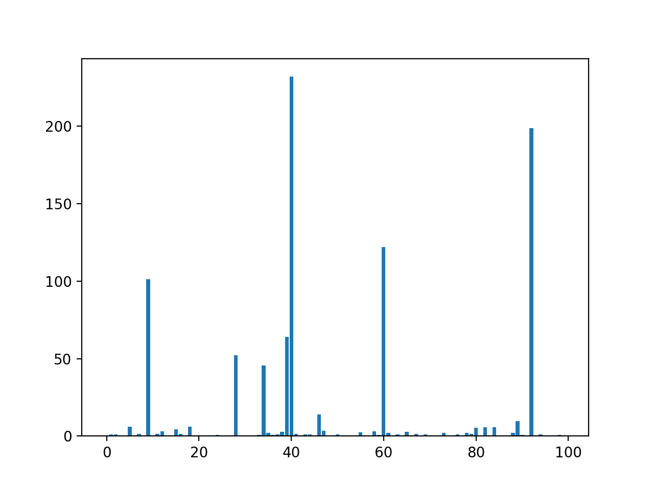
Bar Chart of the Input Features (x) vs. Correlation Feature Importance (y)
Mutual Information Feature Selection
Mutual information from the field of information theory is the application of information gain (typically used in the construction of decision trees) to feature selection.
Mutual information is calculated between two variables and measures the reduction in uncertainty for one variable given a known value of the other variable.
You can learn more about mutual information in the following tutorial.
Mutual information is straightforward when considering the distribution of two discrete (categorical or ordinal) variables, such as categorical input and categorical output data. Nevertheless, it can be adapted for use with numerical input and output data.
For technical details on how this can be achieved, see the 2014 paper titled “Mutual Information between Discrete and Continuous Data Sets.”
The scikit-learn machine learning library provides an implementation of mutual information for feature selection with numeric input and output variables via the mutual_info_regression() function.
Like f_regression(), it can be used in the SelectKBest feature selection strategy (and other strategies).
...
# configure to select all features
fs = SelectKBest(score_func=mutual_info_regression, k='all')
# learn relationship from training data
fs.fit(X_train, y_train)
# transform train input data
X_train_fs = fs.transform(X_train)
# transform test input data
X_test_fs = fs.transform(X_test)
return X_train_fs, X_test_fs, fs
We can perform feature selection using mutual information on the dataset and print and plot the scores (larger is better) as we did in the previous section.
The complete example of using mutual information for numerical feature selection is listed below.
# example of mutual information feature selection for numerical input data
from sklearn.datasets import make_regression
from sklearn.model_selection import train_test_split
from sklearn.feature_selection import SelectKBest
from sklearn.feature_selection import mutual_info_regression
from matplotlib import pyplot

# feature selection
def select_features(X_train, y_train, X_test):
	# configure to select all features
	fs = SelectKBest(score_func=mutual_info_regression, k='all')
	# learn relationship from training data
	fs.fit(X_train, y_train)
	# transform train input data
	X_train_fs = fs.transform(X_train)
	# transform test input data
	X_test_fs = fs.transform(X_test)
	return X_train_fs, X_test_fs, fs

# load the dataset
X, y = make_regression(n_samples=1000, n_features=100, n_informative=10, noise=0.1, random_state=1)
# split into train and test sets
X_train, X_test, y_train, y_test = train_test_split(X, y, test_size=0.33, random_state=1)
# feature selection
X_train_fs, X_test_fs, fs = select_features(X_train, y_train, X_test)
# what are scores for the features
for i in range(len(fs.scores_)):
	print('Feature %d: %f' % (i, fs.scores_[i]))
# plot the scores
pyplot.bar([i for i in range(len(fs.scores_))], fs.scores_)
pyplot.show()
Running the example first prints the scores calculated for each input feature and the target variable.
Note that your specific results may vary. Try running the example a few times.
Again, we will not list the scores for all 100 input variables. We can see many features have a score of 0.0, whereas this technique has identified many more features that may be relevant to the target.
Feature 0: 0.045484
Feature 1: 0.000000
Feature 2: 0.000000
Feature 3: 0.000000
Feature 4: 0.024816
Feature 5: 0.000000
Feature 6: 0.022659
Feature 7: 0.000000
Feature 8: 0.000000
Feature 9: 0.074320
...
A bar chart of the feature importance scores for each input feature is created.
Compared to the correlation feature selection method we can clearly see many more features scored as being relevant. This may be because of the statistical noise that we added to the dataset in its construction.
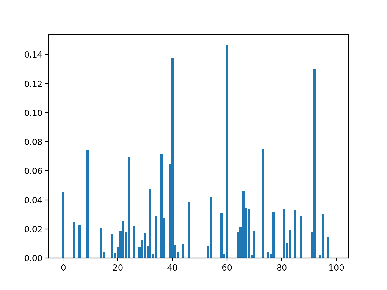
Bar Chart of the Input Features (x) vs. the Mutual Information Feature Importance (y)
Now that we know how to perform feature selection on numerical input data for a regression predictive modeling problem, we can try developing a model using the selected features and compare the results.
Modeling With Selected Features
There are many different techniques for scoring features and selecting features based on scores; how do you know which one to use?
A robust approach is to evaluate models using different feature selection methods (and numbers of features) and select the method that results in a model with the best performance.
In this section, we will evaluate a Linear Regression model with all features compared to a model built from features selected by correlation statistics and those features selected via mutual information.
Linear regression is a good model for testing feature selection methods as it can perform better if irrelevant features are removed from the model.
Model Built Using All Features
As a first step, we will evaluate a LinearRegression model using all the available features.
The model is fit on the training dataset and evaluated on the test dataset.
The complete example is listed below.
# evaluation of a model using all input features
from sklearn.datasets import make_regression
from sklearn.model_selection import train_test_split
from sklearn.linear_model import LinearRegression
from sklearn.metrics import mean_absolute_error
# load the dataset
X, y = make_regression(n_samples=1000, n_features=100, n_informative=10, noise=0.1, random_state=1)
# split into train and test sets
X_train, X_test, y_train, y_test = train_test_split(X, y, test_size=0.33, random_state=1)
# fit the model
model = LinearRegression()
model.fit(X_train, y_train)
# evaluate the model
yhat = model.predict(X_test)
# evaluate predictions
mae = mean_absolute_error(y_test, yhat)
print('MAE: %.3f' % mae)
Running the example prints the mean absolute error (MAE) of the model on the training dataset.
Note that your specific results may vary given the stochastic nature of the learning algorithm. Try running the example a few times.
In this case, we can see that the model achieves an error of about 0.086.
We would prefer to use a subset of features that achieves an error that is as good or better than this.
MAE: 0.086
Model Built Using Correlation Features
We can use the correlation method to score the features and select the 10 most relevant ones.
The select_features() function below is updated to achieve this.
# feature selection
def select_features(X_train, y_train, X_test):
	# configure to select a subset of features
	fs = SelectKBest(score_func=f_regression, k=10)
	# learn relationship from training data
	fs.fit(X_train, y_train)
	# transform train input data
	X_train_fs = fs.transform(X_train)
	# transform test input data
	X_test_fs = fs.transform(X_test)
	return X_train_fs, X_test_fs, fs
The complete example of evaluating a linear regression model fit and evaluated on data using this feature selection method is listed below.
# evaluation of a model using 10 features chosen with correlation
from sklearn.datasets import make_regression
from sklearn.model_selection import train_test_split
from sklearn.feature_selection import SelectKBest
from sklearn.feature_selection import f_regression
from sklearn.linear_model import LinearRegression
from sklearn.metrics import mean_absolute_error

# feature selection
def select_features(X_train, y_train, X_test):
	# configure to select a subset of features
	fs = SelectKBest(score_func=f_regression, k=10)
	# learn relationship from training data
	fs.fit(X_train, y_train)
	# transform train input data
	X_train_fs = fs.transform(X_train)
	# transform test input data
	X_test_fs = fs.transform(X_test)
	return X_train_fs, X_test_fs, fs

# load the dataset
X, y = make_regression(n_samples=1000, n_features=100, n_informative=10, noise=0.1, random_state=1)
# split into train and test sets
X_train, X_test, y_train, y_test = train_test_split(X, y, test_size=0.33, random_state=1)
# feature selection
X_train_fs, X_test_fs, fs = select_features(X_train, y_train, X_test)
# fit the model
model = LinearRegression()
model.fit(X_train_fs, y_train)
# evaluate the model
yhat = model.predict(X_test_fs)
# evaluate predictions
mae = mean_absolute_error(y_test, yhat)
print('MAE: %.3f' % mae)
Running the example reports the performance of the model on just 10 of the 100 input features selected using the correlation statistic.
Note that your specific results may vary given the stochastic nature of the learning algorithm. Try running the example a few times.
In this case, we see that the model achieved an error score of about 2.7, which is much larger than the baseline model that used all features and achieved an MAE of 0.086.
This suggests that although the method has a strong idea of what features to select, building a model from these features alone does not result in a more skillful model. This could be because features that are important to the target are being left out, meaning that the method is being deceived about what is important.
MAE: 2.740
Let’s go the other way and try to use the method to remove some redundant features rather than all redundant features.
We can do this by setting the number of selected features to a much larger value, in this case, 88, hoping it can find and discard 12 of the 90 redundant features.
The complete example is listed below.
# evaluation of a model using 88 features chosen with correlation
from sklearn.datasets import make_regression
from sklearn.model_selection import train_test_split
from sklearn.feature_selection import SelectKBest
from sklearn.feature_selection import f_regression
from sklearn.linear_model import LinearRegression
from sklearn.metrics import mean_absolute_error

# feature selection
def select_features(X_train, y_train, X_test):
	# configure to select a subset of features
	fs = SelectKBest(score_func=f_regression, k=88)
	# learn relationship from training data
	fs.fit(X_train, y_train)
	# transform train input data
	X_train_fs = fs.transform(X_train)
	# transform test input data
	X_test_fs = fs.transform(X_test)
	return X_train_fs, X_test_fs, fs

# load the dataset
X, y = make_regression(n_samples=1000, n_features=100, n_informative=10, noise=0.1, random_state=1)
# split into train and test sets
X_train, X_test, y_train, y_test = train_test_split(X, y, test_size=0.33, random_state=1)
# feature selection
X_train_fs, X_test_fs, fs = select_features(X_train, y_train, X_test)
# fit the model
model = LinearRegression()
model.fit(X_train_fs, y_train)
# evaluate the model
yhat = model.predict(X_test_fs)
# evaluate predictions
mae = mean_absolute_error(y_test, yhat)
print('MAE: %.3f' % mae)
Running the example reports the performance of the model on 88 of the 100 input features selected using the correlation statistic.
Note that your specific results may vary given the stochastic nature of the learning algorithm. Try running the example a few times.
In this case, we can see that removing some of the redundant features has resulted in a small lift in performance with an error of about 0.085 compared to the baseline that achieved an error of about 0.086.
MAE: 0.085
Model Built Using Mutual Information Features
We can repeat the experiment and select the top 88 features using a mutual information statistic.
The updated version of the select_features() function to achieve this is listed below.
# feature selection
def select_features(X_train, y_train, X_test):
	# configure to select a subset of features
	fs = SelectKBest(score_func=mutual_info_regression, k=88)
	# learn relationship from training data
	fs.fit(X_train, y_train)
	# transform train input data
	X_train_fs = fs.transform(X_train)
	# transform test input data
	X_test_fs = fs.transform(X_test)
	return X_train_fs, X_test_fs, fs
The complete example of using mutual information for feature selection to fit a linear regression model is listed below.
# evaluation of a model using 88 features chosen with mutual information
from sklearn.datasets import make_regression
from sklearn.model_selection import train_test_split
from sklearn.feature_selection import SelectKBest
from sklearn.feature_selection import mutual_info_regression
from sklearn.linear_model import LinearRegression
from sklearn.metrics import mean_absolute_error

# feature selection
def select_features(X_train, y_train, X_test):
	# configure to select a subset of features
	fs = SelectKBest(score_func=mutual_info_regression, k=88)
	# learn relationship from training data
	fs.fit(X_train, y_train)
	# transform train input data
	X_train_fs = fs.transform(X_train)
	# transform test input data
	X_test_fs = fs.transform(X_test)
	return X_train_fs, X_test_fs, fs

# load the dataset
X, y = make_regression(n_samples=1000, n_features=100, n_informative=10, noise=0.1, random_state=1)
# split into train and test sets
X_train, X_test, y_train, y_test = train_test_split(X, y, test_size=0.33, random_state=1)
# feature selection
X_train_fs, X_test_fs, fs = select_features(X_train, y_train, X_test)
# fit the model
model = LinearRegression()
model.fit(X_train_fs, y_train)
# evaluate the model
yhat = model.predict(X_test_fs)
# evaluate predictions
mae = mean_absolute_error(y_test, yhat)
print('MAE: %.3f' % mae)
Running the example fits the model on the 88 top selected features chosen using mutual information.
Note: your specific results may vary given the stochastic nature of the learning algorithm. Try running the example a few times.
In this case, we can see a further reduction in error as compared to the correlation statistic, in this case, achieving a MAE of about 0.084 compared to 0.085 in the previous section.
MAE: 0.084
Tune the Number of Selected Features
In the previous example, we selected 88 features, but how do we know that is a good or best number of features to select?
Instead of guessing, we can systematically test a range of different numbers of selected features and discover which results in the best performing model. This is called a grid search, where the k argument to the SelectKBest class can be tuned.
It is a good practice to evaluate model configurations on regression tasks using repeated stratified k-fold cross-validation. We will use three repeats of 10-fold cross-validation via the RepeatedKFold class.
...
# define the evaluation method
cv = RepeatedKFold(n_splits=10, n_repeats=3, random_state=1)
We can define a Pipeline that correctly prepares the feature selection transform on the training set and applies it to the train set and test set for each fold of the cross-validation.
In this case, we will use the mutual information statistical method for selecting features.
...
# define the pipeline to evaluate
model = LinearRegression()
fs = SelectKBest(score_func=mutual_info_regression)
pipeline = Pipeline(steps=[('sel',fs), ('lr', model)])
We can then define the grid of values to evaluate as 80 to 100.
Note that the grid is a dictionary mapping of parameter-to-values to search, and given that we are using a Pipeline, we can access the SelectKBest object via the name we gave it ‘sel‘ and then the parameter name ‘k‘ separated by two underscores, or ‘sel__k‘.
...
# define the grid
grid = dict()
grid['sel__k'] = [i for i in range(X.shape[1]-20, X.shape[1]+1)]
We can then define and run the search.
In this case, we will evaluate models using the negative mean absolute error (neg_mean_absolute_error). It is negative because the scikit-learn requires the score to be maximized, so the MAE is made negative, meaning scores scale from -infinity to 0 (best).
...
# define the grid search
search = GridSearchCV(pipeline, grid, scoring='neg_mean_absolure_error', n_jobs=-1, cv=cv)
# perform the search
results = search.fit(X, y)
Tying this together, the complete example is listed below.
# compare different numbers of features selected using mutual information
from sklearn.datasets import make_regression
from sklearn.model_selection import RepeatedKFold
from sklearn.feature_selection import SelectKBest
from sklearn.feature_selection import mutual_info_regression
from sklearn.linear_model import LinearRegression
from sklearn.pipeline import Pipeline
from sklearn.model_selection import GridSearchCV
# define dataset
X, y = make_regression(n_samples=1000, n_features=100, n_informative=10, noise=0.1, random_state=1)
# define the evaluation method
cv = RepeatedKFold(n_splits=10, n_repeats=3, random_state=1)
# define the pipeline to evaluate
model = LinearRegression()
fs = SelectKBest(score_func=mutual_info_regression)
pipeline = Pipeline(steps=[('sel',fs), ('lr', model)])
# define the grid
grid = dict()
grid['sel__k'] = [i for i in range(X.shape[1]-20, X.shape[1]+1)]
# define the grid search
search = GridSearchCV(pipeline, grid, scoring='neg_mean_squared_error', n_jobs=-1, cv=cv)
# perform the search
results = search.fit(X, y)
# summarize best
print('Best MAE: %.3f' % results.best_score_)
print('Best Config: %s' % results.best_params_)
# summarize all
means = results.cv_results_['mean_test_score']
params = results.cv_results_['params']
for mean, param in zip(means, params):
    print(">%.3f with: %r" % (mean, param))
Running the example grid searches different numbers of selected features using mutual information statistics, where each modeling pipeline is evaluated using repeated cross-validation.
Your specific results may vary given the stochastic nature of the learning algorithm and evaluating procedure. Try running the example a few times.
In this case, we can see that the best number of selected features is 81, which achieves a MAE of about 0.082 (ignoring the sign).
Best MAE: -0.082
Best Config: {'sel__k': 81}
>-1.100 with: {'sel__k': 80}
>-0.082 with: {'sel__k': 81}
>-0.082 with: {'sel__k': 82}
>-0.082 with: {'sel__k': 83}
>-0.082 with: {'sel__k': 84}
>-0.082 with: {'sel__k': 85}
>-0.082 with: {'sel__k': 86}
>-0.082 with: {'sel__k': 87}
>-0.082 with: {'sel__k': 88}
>-0.083 with: {'sel__k': 89}
>-0.083 with: {'sel__k': 90}
>-0.083 with: {'sel__k': 91}
>-0.083 with: {'sel__k': 92}
>-0.083 with: {'sel__k': 93}
>-0.083 with: {'sel__k': 94}
>-0.083 with: {'sel__k': 95}
>-0.083 with: {'sel__k': 96}
>-0.083 with: {'sel__k': 97}
>-0.083 with: {'sel__k': 98}
>-0.083 with: {'sel__k': 99}
>-0.083 with: {'sel__k': 100}
We might want to see the relationship between the number of selected features and MAE. In this relationship, we may expect that more features result in better performance, to a point.
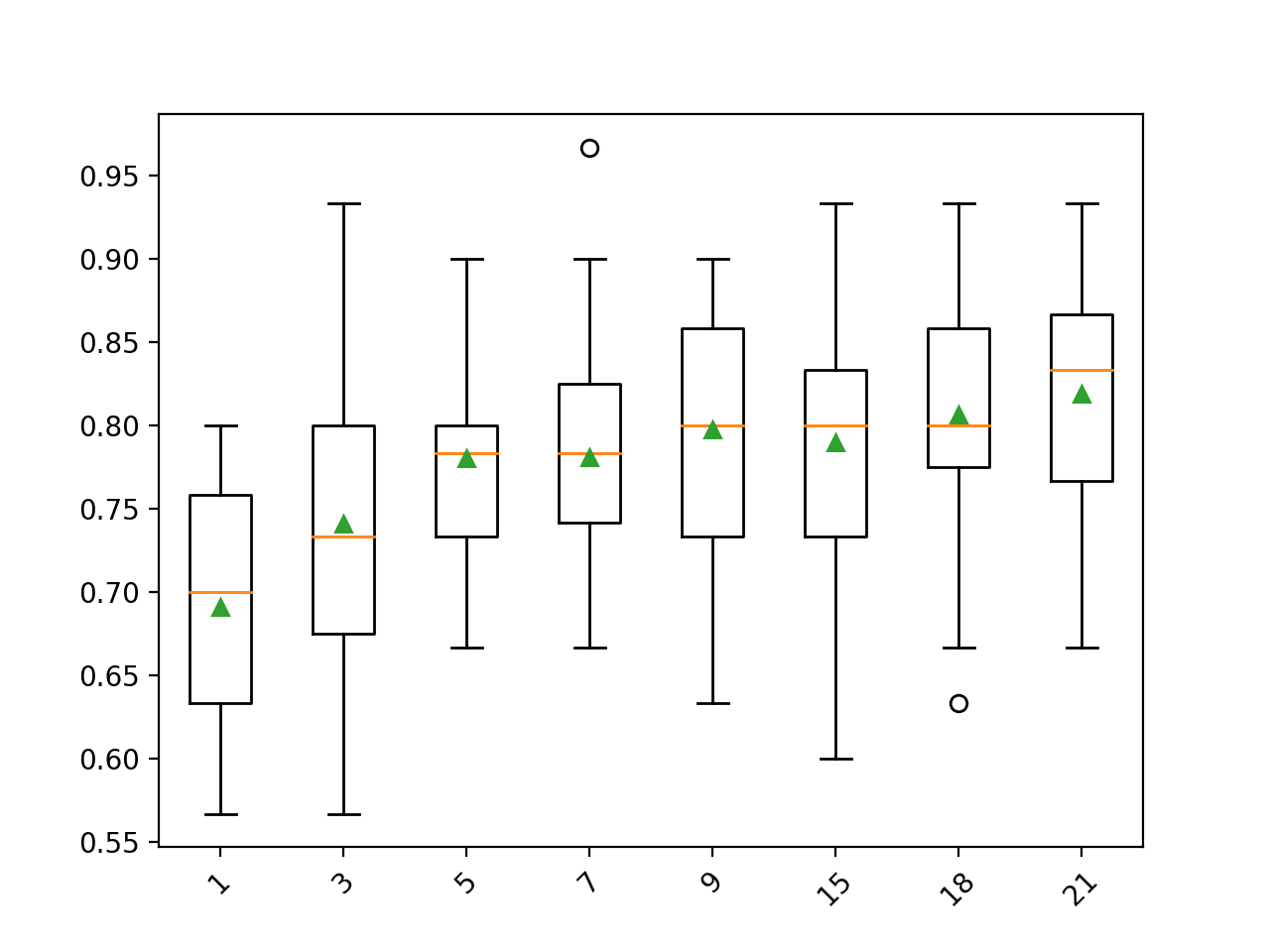
This relationship can be explored by manually evaluating each configuration of k for the SelectKBest from 81 to 100, gathering the sample of MAE scores, and plotting the results using box and whisker plots side by side. The spread and mean of these box plots would be expected to show any interesting relationship between the number of selected features and the MAE of the pipeline.
Note that we started the spread of k values at 81 instead of 80 because the distribution of MAE scores for k=80 is dramatically larger than all other values of k considered and it washed out the plot of the results on the graph.
The complete example of achieving this is listed below.
# compare different numbers of features selected using mutual information
from numpy import mean
from numpy import std
from sklearn.datasets import make_regression
from sklearn.model_selection import cross_val_score
from sklearn.model_selection import RepeatedKFold
from sklearn.feature_selection import SelectKBest
from sklearn.feature_selection import mutual_info_regression
from sklearn.linear_model import LinearRegression
from sklearn.pipeline import Pipeline
from matplotlib import pyplot
# define dataset
X, y = make_regression(n_samples=1000, n_features=100, n_informative=10, noise=0.1, random_state=1)
# define number of features to evaluate
num_features = [i for i in range(X.shape[1]-19, X.shape[1]+1)]
# enumerate each number of features
results = list()
for k in num_features:
	# create pipeline
	model = LinearRegression()
	fs = SelectKBest(score_func=mutual_info_regression, k=k)
	pipeline = Pipeline(steps=[('sel',fs), ('lr', model)])
	# evaluate the model
	cv = RepeatedKFold(n_splits=10, n_repeats=3, random_state=1)
	scores = cross_val_score(pipeline, X, y, scoring='neg_mean_absolute_error', cv=cv, n_jobs=-1)
	results.append(scores)
	# summarize the results
	print('>%d %.3f (%.3f)' % (k, mean(scores), std(scores)))
# plot model performance for comparison
pyplot.boxplot(results, labels=num_features, showmeans=True)
pyplot.show()
Running the example first reports the mean and standard deviation MAE for each number of selected features.
Your specific results may vary given the stochastic nature of the learning algorithm and evaluating procedure. Try running the example a few times.
In this case, reporting the mean and standard deviation of MAE is not very interesting, other than values of k in the 80s appear better than those in the 90s.
>81 -0.082 (0.006)
>82 -0.082 (0.006)
>83 -0.082 (0.006)
>84 -0.082 (0.006)
>85 -0.082 (0.006)
>86 -0.082 (0.006)
>87 -0.082 (0.006)
>88 -0.082 (0.006)
>89 -0.083 (0.006)
>90 -0.083 (0.006)
>91 -0.083 (0.006)
>92 -0.083 (0.006)
>93 -0.083 (0.006)
>94 -0.083 (0.006)
>95 -0.083 (0.006)
>96 -0.083 (0.006)
>97 -0.083 (0.006)
>98 -0.083 (0.006)
>99 -0.083 (0.006)
>100 -0.083 (0.006)
Box and whisker plots are created side by side showing the trend of k vs. MAE where the green triangle represents the mean and orange line represents the median of the distribution.
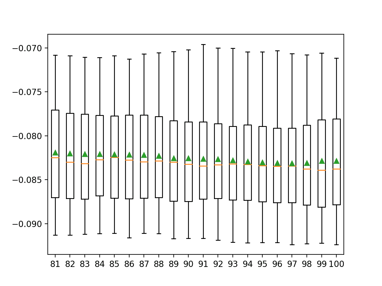
Box and Whisker Plots of MAE for Each Number of Selected Features Using Mutual Information
Further Reading
This section provides more resources on the topic if you are looking to go deeper.
Tutorials
- How to Choose a Feature Selection Method For Machine Learning
- How to Perform Feature Selection with Categorical Data
- How to Calculate Correlation Between Variables in Python
- What Is Information Gain and Mutual Information for Machine Learning
Books
- Applied Predictive Modeling, 2013.
APIs
- Feature selection, Scikit-Learn User Guide.
- sklearn.datasets.make_regression API.
- sklearn.feature_selection.f_regression API.
- sklearn.feature_selection.mutual_info_regression API.
Articles
Summary
In this tutorial, you discovered how to perform feature selection with numerical input data for regression predictive modeling.
Specifically, you learned:
- How to evaluate the importance of numerical input data using the correlation and mutual information statistics.
- How to perform feature selection for numerical input data when fitting and evaluating a regression model.
- How to tune the number of features selected in a modeling pipeline using a grid search.
Do you have any questions?
Ask your questions in the comments below and I will do my best to answer.
The post How to Perform Feature Selection for Regression Data appeared first on Machine Learning Mastery.