The Perceptron is a linear machine learning algorithm for binary classification tasks.
It may be considered one of the first and one of the simplest types of artificial neural networks. It is definitely not “deep” learning but is an important building block.
Like logistic regression, it can quickly learn a linear separation in feature space for two-class classification tasks, although unlike logistic regression, it learns using the stochastic gradient descent optimization algorithm and does not predict calibrated probabilities.
In this tutorial, you will discover the Perceptron classification machine learning algorithm.
After completing this tutorial, you will know:
- The Perceptron Classifier is a linear algorithm that can be applied to binary classification tasks.
- How to fit, evaluate, and make predictions with the Perceptron model with Scikit-Learn.
- How to tune the hyperparameters of the Perceptron algorithm on a given dataset.
Let’s get started.

Perceptron Algorithm for Classification in Python
Photo by Belinda Novika, some rights reserved.
Tutorial Overview
This tutorial is divided into 3=three parts; they are:
- Perceptron Algorithm
- Perceptron With Scikit-Learn
- Tune Perceptron Hyperparameters
Perceptron Algorithm
The Perceptron algorithm is a two-class (binary) classification machine learning algorithm.
It is a type of neural network model, perhaps the simplest type of neural network model.
It consists of a single node or neuron that takes a row of data as input and predicts a class label. This is achieved by calculating the weighted sum of the inputs and a bias (set to 1). The weighted sum of the input of the model is called the activation.
- Activation = Weights * Inputs + Bias
If the activation is above 0.0, the model will output 1.0; otherwise, it will output 0.0.
- Predict 1: If Activation > 0.0
- Predict 0: If Activation <= 0.0
Given that the inputs are multiplied by model coefficients, like linear regression and logistic regression, it is good practice to normalize or standardize data prior to using the model.
The Perceptron is a linear classification algorithm. This means that it learns a decision boundary that separates two classes using a line (called a hyperplane) in the feature space. As such, it is appropriate for those problems where the classes can be separated well by a line or linear model, referred to as linearly separable.
The coefficients of the model are referred to as input weights and are trained using the stochastic gradient descent optimization algorithm.
Examples from the training dataset are shown to the model one at a time, the model makes a prediction, and error is calculated. The weights of the model are then updated to reduce the errors for the example. This is called the Perceptron update rule. This process is repeated for all examples in the training dataset, called an epoch. This process of updating the model using examples is then repeated for many epochs.
Model weights are updated with a small proportion of the error each batch, and the proportion is controlled by a hyperparameter called the learning rate, typically set to a small value. This is to ensure learning does not occur too quickly, resulting in a possibly lower skill model, referred to as premature convergence of the optimization (search) procedure for the model weights.
- weights(t + 1) = weights(t) + learning_rate * (expected_i – predicted_) * input_i
Training is stopped when the error made by the model falls to a low level or no longer improves, or a maximum number of epochs is performed.
The initial values for the model weights are set to small random values. Additionally, the training dataset is shuffled prior to each training epoch. This is by design to accelerate and improve the model training process. Because of this, the learning algorithm is stochastic and may achieve different results each time it is run. As such, it is good practice to summarize the performance of the algorithm on a dataset using repeated evaluation and reporting the mean classification accuracy.
The learning rate and number of training epochs are hyperparameters of the algorithm that can be set using heuristics or hyperparameter tuning.
For more about the Perceptron algorithm, see the tutorial:
Now that we are familiar with the Perceptron algorithm, let’s explore how we can use the algorithm in Python.
Perceptron With Scikit-Learn
The Perceptron algorithm is available in the scikit-learn Python machine learning library via the Perceptron class.
The class allows you to configure the learning rate (eta0), which defaults to 1.0.
...
# define model
model = Perceptron(eta0=1.0)
The implementation also allows you to configure the total number of training epochs (max_iter), which defaults to 1,000.
...
# define model
model = Perceptron(max_iter=1000)
The scikit-learn implementation of the Perceptron algorithm also provides other configuration options that you may want to explore, such as early stopping and the use of a penalty loss.
We can demonstrate the Perceptron classifier with a worked example.
First, let’s define a synthetic classification dataset.
We will use the make_classification() function to create a dataset with 1,000 examples, each with 20 input variables.
The example creates and summarizes the dataset.
# test classification dataset
from sklearn.datasets import make_classification
# define dataset
X, y = make_classification(n_samples=1000, n_features=10, n_informative=10, n_redundant=0, random_state=1)
# summarize the dataset
print(X.shape, y.shape)
Running the example creates the dataset and confirms the number of rows and columns of the dataset.
(1000, 10) (1000,)
We can fit and evaluate a Perceptron model using repeated stratified k-fold cross-validation via the RepeatedStratifiedKFold class. We will use 10 folds and three repeats in the test harness.
We will use the default configuration.
...
# create the model
model = Perceptron()
The complete example of evaluating the Perceptron model for the synthetic binary classification task is listed below.
# evaluate a perceptron model on the dataset
from numpy import mean
from numpy import std
from sklearn.datasets import make_classification
from sklearn.model_selection import cross_val_score
from sklearn.model_selection import RepeatedStratifiedKFold
from sklearn.linear_model import Perceptron
# define dataset
X, y = make_classification(n_samples=1000, n_features=10, n_informative=10, n_redundant=0, random_state=1)
# define model
model = Perceptron()
# define model evaluation method
cv = RepeatedStratifiedKFold(n_splits=10, n_repeats=3, random_state=1)
# evaluate model
scores = cross_val_score(model, X, y, scoring='accuracy', cv=cv, n_jobs=-1)
# summarize result
print('Mean Accuracy: %.3f (%.3f)' % (mean(scores), std(scores)))
Running the example evaluates the Perceptron algorithm on the synthetic dataset and reports the average accuracy across the three repeats of 10-fold cross-validation.
Your specific results may vary given the stochastic nature of the learning algorithm. Consider running the example a few times.
In this case, we can see that the model achieved a mean accuracy of about 84.7 percent.
Mean Accuracy: 0.847 (0.052)
We may decide to use the Perceptron classifier as our final model and make predictions on new data.
This can be achieved by fitting the model pipeline on all available data and calling the predict() function passing in a new row of data.
We can demonstrate this with a complete example listed below.
# make a prediction with a perceptron model on the dataset
from sklearn.datasets import make_classification
from sklearn.linear_model import Perceptron
# define dataset
X, y = make_classification(n_samples=1000, n_features=10, n_informative=10, n_redundant=0, random_state=1)
# define model
model = Perceptron()
# fit model
model.fit(X, y)
# define new data
row = [0.12777556,-3.64400522,-2.23268854,-1.82114386,1.75466361,0.1243966,1.03397657,2.35822076,1.01001752,0.56768485]
# make a prediction
yhat = model.predict([row])
# summarize prediction
print('Predicted Class: %d' % yhat)
Running the example fits the model and makes a class label prediction for a new row of data.
Predicted Class: 1
Next, we can look at configuring the model hyperparameters.
Tune Perceptron Hyperparameters
The hyperparameters for the Perceptron algorithm must be configured for your specific dataset.
Perhaps the most important hyperparameter is the learning rate.
A large learning rate can cause the model to learn fast, but perhaps at the cost of lower skill. A smaller learning rate can result in a better-performing model but may take a long time to train the model.
You can learn more about exploring learning rates in the tutorial:
It is common to test learning rates on a log scale between a small value such as 1e-4 (or smaller) and 1.0. We will test the following values in this case:
...
# define grid
grid = dict()
grid['eta0'] = [0.0001, 0.001, 0.01, 0.1, 1.0]
The example below demonstrates this using the GridSearchCV class with a grid of values we have defined.
# grid search learning rate for the perceptron
from sklearn.datasets import make_classification
from sklearn.model_selection import GridSearchCV
from sklearn.model_selection import RepeatedStratifiedKFold
from sklearn.linear_model import Perceptron
# define dataset
X, y = make_classification(n_samples=1000, n_features=10, n_informative=10, n_redundant=0, random_state=1)
# define model
model = Perceptron()
# define model evaluation method
cv = RepeatedStratifiedKFold(n_splits=10, n_repeats=3, random_state=1)
# define grid
grid = dict()
grid['eta0'] = [0.0001, 0.001, 0.01, 0.1, 1.0]
# define search
search = GridSearchCV(model, grid, scoring='accuracy', cv=cv, n_jobs=-1)
# perform the search
results = search.fit(X, y)
# summarize
print('Mean Accuracy: %.3f' % results.best_score_)
print('Config: %s' % results.best_params_)
# summarize all
means = results.cv_results_['mean_test_score']
params = results.cv_results_['params']
for mean, param in zip(means, params):
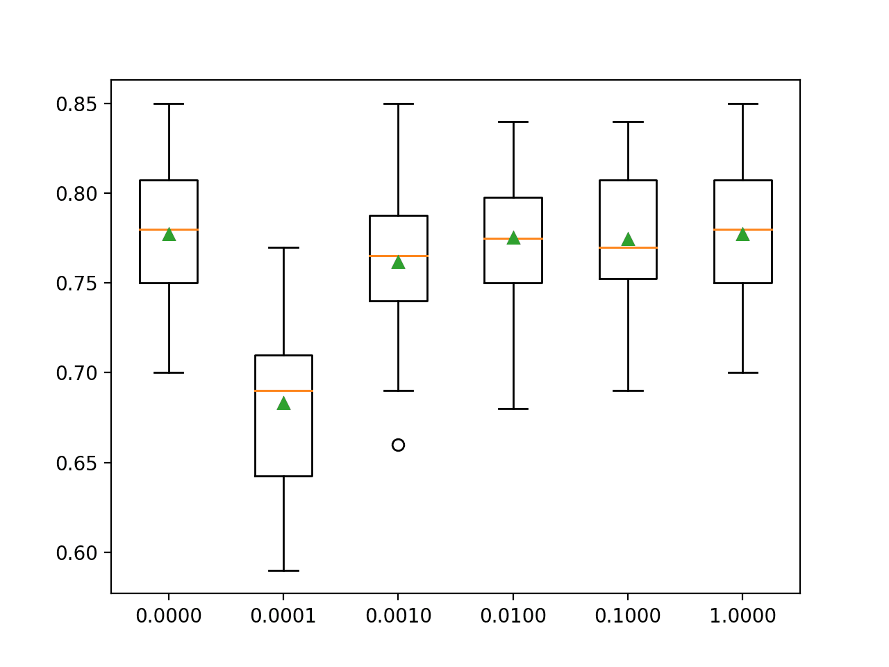
print(">%.3f with: %r" % (mean, param))Running the example will evaluate each combination of configurations using repeated cross-validation.
Your specific results may vary given the stochastic nature of the learning algorithm. Try running the example a few times.
In this case, we can see that a smaller learning rate than the default results in better performance with learning rate 0.0001 and 0.001 both achieving a classification accuracy of about 85.7 percent as compared to the default of 1.0 that achieved an accuracy of about 84.7 percent.
Mean Accuracy: 0.857
Config: {'eta0': 0.0001}
>0.857 with: {'eta0': 0.0001}
>0.857 with: {'eta0': 0.001}
>0.853 with: {'eta0': 0.01}
>0.847 with: {'eta0': 0.1}
>0.847 with: {'eta0': 1.0}
Another important hyperparameter is how many epochs are used to train the model.
This may depend on the training dataset and could vary greatly. Again, we will explore configuration values on a log scale between 1 and 1e+4.
...
# define grid
grid = dict()
grid['max_iter'] = [1, 10, 100, 1000, 10000]
We will use our well-performing learning rate of 0.0001 found in the previous search.
...
# define model
model = Perceptron(eta0=0.0001)
The complete example of grid searching the number of training epochs is listed below.
# grid search total epochs for the perceptron
from sklearn.datasets import make_classification
from sklearn.model_selection import GridSearchCV
from sklearn.model_selection import RepeatedStratifiedKFold
from sklearn.linear_model import Perceptron
# define dataset
X, y = make_classification(n_samples=1000, n_features=10, n_informative=10, n_redundant=0, random_state=1)
# define model
model = Perceptron(eta0=0.0001)
# define model evaluation method
cv = RepeatedStratifiedKFold(n_splits=10, n_repeats=3, random_state=1)
# define grid
grid = dict()
grid['max_iter'] = [1, 10, 100, 1000, 10000]
# define search
search = GridSearchCV(model, grid, scoring='accuracy', cv=cv, n_jobs=-1)
# perform the search
results = search.fit(X, y)
# summarize
print('Mean Accuracy: %.3f' % results.best_score_)
print('Config: %s' % results.best_params_)
# summarize all
means = results.cv_results_['mean_test_score']
params = results.cv_results_['params']
for mean, param in zip(means, params):
    print(">%.3f with: %r" % (mean, param))
Running the example will evaluate each combination of configurations using repeated cross-validation.
Your specific results may vary given the stochastic nature of the learning algorithm. Try running the example a few times.
In this case, we can see that epochs 10 to 10,000 result in about the same classification accuracy. An interesting exception would be to explore configuring learning rate and number of training epochs at the same time to see if better results can be achieved.
Mean Accuracy: 0.857
Config: {'max_iter': 10}
>0.850 with: {'max_iter': 1}
>0.857 with: {'max_iter': 10}
>0.857 with: {'max_iter': 100}
>0.857 with: {'max_iter': 1000}
>0.857 with: {'max_iter': 10000}
Further Reading
This section provides more resources on the topic if you are looking to go deeper.
Tutorials
- How To Implement The Perceptron Algorithm From Scratch In Python
- Understand the Impact of Learning Rate on Neural Network Performance
- How to Configure the Learning Rate When Training Deep Learning Neural Networks
Books
- Neural Networks for Pattern Recognition, 1995.
- Pattern Recognition and Machine Learning, 2006.
- Artificial Intelligence: A Modern Approach, 3rd edition, 2015.
APIs
Articles
Summary
In this tutorial, you discovered the Perceptron classification machine learning algorithm.
Specifically, you learned:
- The Perceptron Classifier is a linear algorithm that can be applied to binary classification tasks.
- How to fit, evaluate, and make predictions with the Perceptron model with Scikit-Learn.
- How to tune the hyperparameters of the Perceptron algorithm on a given dataset.
Do you have any questions?
Ask your questions in the comments below and I will do my best to answer.
The post Perceptron Algorithm for Classification in Python appeared first on Machine Learning Mastery.