Developing a neural network predictive model for a new dataset can be challenging.
One approach is to first inspect the dataset and develop ideas for what models might work, then explore the learning dynamics of simple models on the dataset, then finally develop and tune a model for the dataset with a robust test harness.
This process can be used to develop effective neural network models for classification and regression predictive modeling problems.
In this tutorial, you will discover how to develop a Multilayer Perceptron neural network model for the Swedish car insurance regression dataset.
After completing this tutorial, you will know:
- How to load and summarize the Swedish car insurance dataset and use the results to suggest data preparations and model configurations to use.
- How to explore the learning dynamics of simple MLP models and data transforms on the dataset.
- How to develop robust estimates of model performance, tune model performance, and make predictions on new data.
Let’s get started.

How to Develop a Neural Net for Predicting Car Insurance Payout
Photo by Dimitry B., some rights reserved.
Tutorial Overview
This tutorial is divided into four parts; they are:
- Auto Insurance Regression Dataset
- First MLP and Learning Dynamics
- Evaluating and Tuning MLP Models
- Final Model and Make Predictions
Auto Insurance Regression Dataset
The first step is to define and explore the dataset.
We will be working with the “Auto Insurance” standard regression dataset.
The dataset describes Swedish car insurance. There is a single input variable, which is the number of claims, and the target variable is a total payment for the claims in thousands of Swedish krona. The goal is to predict the total payment given the number of claims.
You can learn more about the dataset here:
You can see the first few rows of the dataset below.
108,392.5
19,46.2
13,15.7
124,422.2
40,119.4
...
We can see that the values are numeric and may range from tens to hundreds. This suggests some type of scaling would be appropriate for the data when modeling with a neural network.
We can load the dataset as a pandas DataFrame directly from the URL; for example:
# load the dataset and summarize the shape
from pandas import read_csv
# define the location of the dataset
url = 'https://raw.githubusercontent.com/jbrownlee/Datasets/master/auto-insurance.csv'
# load the dataset
df = read_csv(url, header=None)
# summarize shape
print(df.shape)
Running the example loads the dataset directly from the URL and reports the shape of the dataset.
In this case, we can confirm that the dataset has two variables (one input and one output) and that the dataset has 63 rows of data.
This is not many rows of data for a neural network and suggests that a small network, perhaps with regularization, would be appropriate.
It also suggests that using k-fold cross-validation would be a good idea given that it will give a more reliable estimate of model performance than a train/test split and because a single model will fit in seconds instead of hours or days with the largest datasets.
(63, 2)
Next, we can learn more about the dataset by looking at summary statistics and a plot of the data.
# show summary statistics and plots of the dataset
from pandas import read_csv
from matplotlib import pyplot
# define the location of the dataset
url = 'https://raw.githubusercontent.com/jbrownlee/Datasets/master/auto-insurance.csv'
# load the dataset
df = read_csv(url, header=None)
# show summary statistics
print(df.describe())
# plot histograms
df.hist()
pyplot.show()
Running the example first loads the data before and then prints summary statistics for each variable
We can see that the mean value for each variable is in the tens, with values ranging from 0 to the hundreds. This confirms that scaling the data is probably a good idea.
0           1
count   63.000000   63.000000
mean    22.904762   98.187302
std     23.351946   87.327553
min      0.000000    0.000000
25%      7.500000   38.850000
50%     14.000000   73.400000
75%     29.000000  140.000000
max    124.000000  422.200000
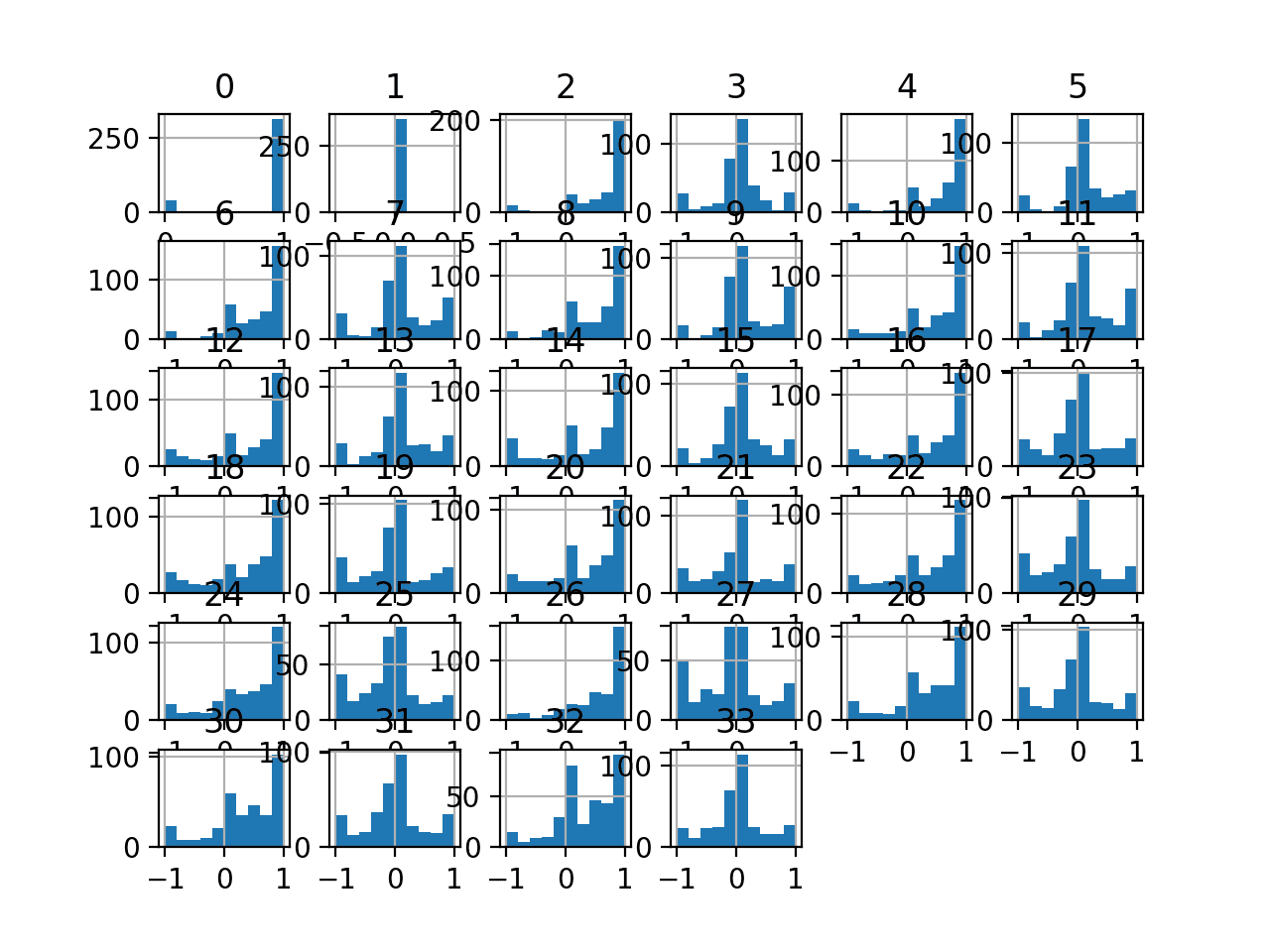
A histogram plot is then created for each variable.
We can see that each variable has a similar distribution. It looks like a skewed Gaussian distribution or an exponential distribution.
We may have some benefit in using a power transform on each variable in order to make the probability distribution less skewed, which will likely improve model performance.
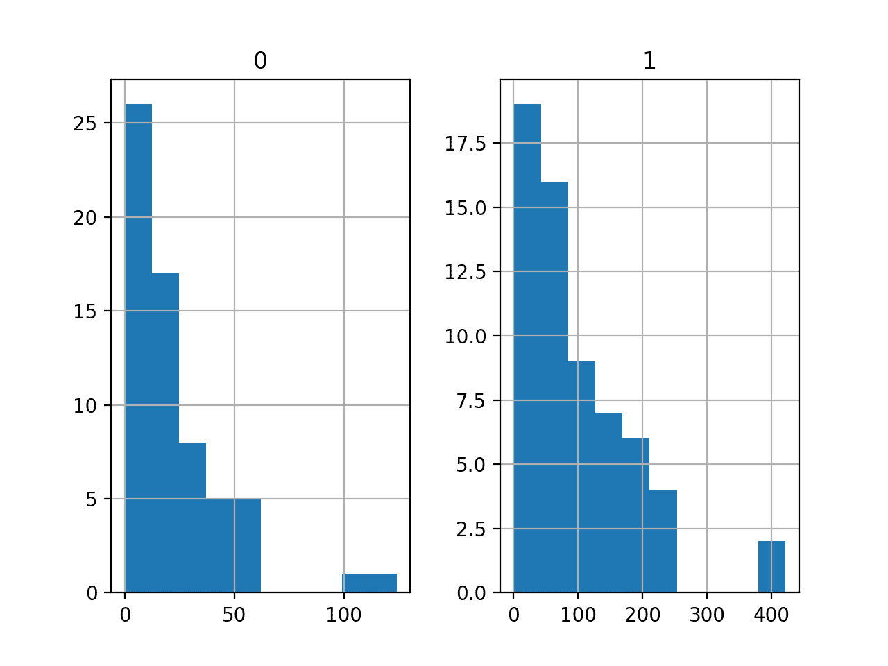
Histograms of the Auto Insurance Regression Dataset
Now that we are familiar with the dataset, let’s explore how we might develop a neural network model.
First MLP and Learning Dynamics
We will develop a Multilayer Perceptron (MLP) model for the dataset using TensorFlow.
We cannot know what model architecture of learning hyperparameters would be good or best for this dataset, so we must experiment and discover what works well.
Given that the dataset is small, a small batch size is probably a good idea, e.g. 8 or 16 rows. Using the Adam version of stochastic gradient descent is a good idea when getting started as it will automatically adapt the learning rate and works well on most datasets.
Before we evaluate models in earnest, it is a good idea to review the learning dynamics and tune the model architecture and learning configuration until we have stable learning dynamics, then look at getting the most out of the model.
We can do this by using a simple train/test split of the data and review plots of the learning curves. This will help us see if we are over-learning or under-learning; then we can adapt the configuration accordingly.
First, we can split the dataset into input and output variables, then into 67/33 train and test sets.
...
# split into input and output columns
X, y = df.values[:, :-1], df.values[:, -1]
# split into train and test datasets
X_train, X_test, y_train, y_test = train_test_split(X, y, test_size=0.33)
Next, we can define a minimal MLP model. In this case, we will use one hidden layer with 10 nodes and one output layer (chosen arbitrarily). We will use the ReLU activation function in the hidden layer and the “he_normal” weight initialization, as together, they are a good practice.
The output of the model is a linear activation (no activation) and we will minimize mean squared error (MSE) loss.
...
# determine the number of input features
n_features = X.shape[1]
# define model
model = Sequential()
model.add(Dense(10, activation='relu', kernel_initializer='he_normal', input_shape=(n_features,)))
model.add(Dense(1))
# compile the model
model.compile(optimizer='adam', loss='mse')
We will fit the model for 100 training epochs (chosen arbitrarily) with a batch size of eight because it is a small dataset.
We are fitting the model on raw data, which we think might be a bad idea, but it is an important starting point.
...
# fit the model
history = model.fit(X_train, y_train, epochs=100, batch_size=8, verbose=0, validation_data=(X_test,y_test))
At the end of training, we will evaluate the model’s performance on the test dataset and report performance as the mean absolute error (MAE), which I typically prefer over MSE or RMSE.
...
# predict test set
yhat = model.predict(X_test)
# evaluate predictions
score = mean_absolute_error(y_test, yhat)
print('MAE: %.3f' % score)
Finally, we will plot learning curves of the MSE loss on the train and test sets during training.
...
# plot learning curves
pyplot.title('Learning Curves')
pyplot.xlabel('Epoch')
pyplot.ylabel('Mean Squared Error')
pyplot.plot(history.history['loss'], label='train')
pyplot.plot(history.history['val_loss'], label='val')
pyplot.legend()
pyplot.show()
Tying this all together, the complete example of evaluating our first MLP on the auto insurance dataset is listed below.
# fit a simple mlp model and review learning curves
from pandas import read_csv
from sklearn.model_selection import train_test_split
from sklearn.metrics import mean_absolute_error
from tensorflow.keras import Sequential
from tensorflow.keras.layers import Dense
from matplotlib import pyplot
# load the dataset
path = 'https://raw.githubusercontent.com/jbrownlee/Datasets/master/auto-insurance.csv'
df = read_csv(path, header=None)
# split into input and output columns
X, y = df.values[:, :-1], df.values[:, -1]
# split into train and test datasets
X_train, X_test, y_train, y_test = train_test_split(X, y, test_size=0.33)
# determine the number of input features
n_features = X.shape[1]
# define model
model = Sequential()
model.add(Dense(10, activation='relu', kernel_initializer='he_normal', input_shape=(n_features,)))
model.add(Dense(1))
# compile the model
model.compile(optimizer='adam', loss='mse')
# fit the model
history = model.fit(X_train, y_train, epochs=100, batch_size=8, verbose=0, validation_data=(X_test,y_test))
# predict test set
yhat = model.predict(X_test)
# evaluate predictions
score = mean_absolute_error(y_test, yhat)
print('MAE: %.3f' % score)
# plot learning curves
pyplot.title('Learning Curves')
pyplot.xlabel('Epoch')
pyplot.ylabel('Mean Squared Error')
pyplot.plot(history.history['loss'], label='train')
pyplot.plot(history.history['val_loss'], label='val')
pyplot.legend()
pyplot.show()
Running the example first fits the model on the training dataset, then reports the MAE on the test dataset.
Note: Your results may vary given the stochastic nature of the algorithm or evaluation procedure, or differences in numerical precision. Consider running the example a few times and compare the average outcome.
In this case, we can see that the model achieved a MAE of about 33.2, which is a good baseline in performance, which we might be able to improve upon.
MAE: 33.233
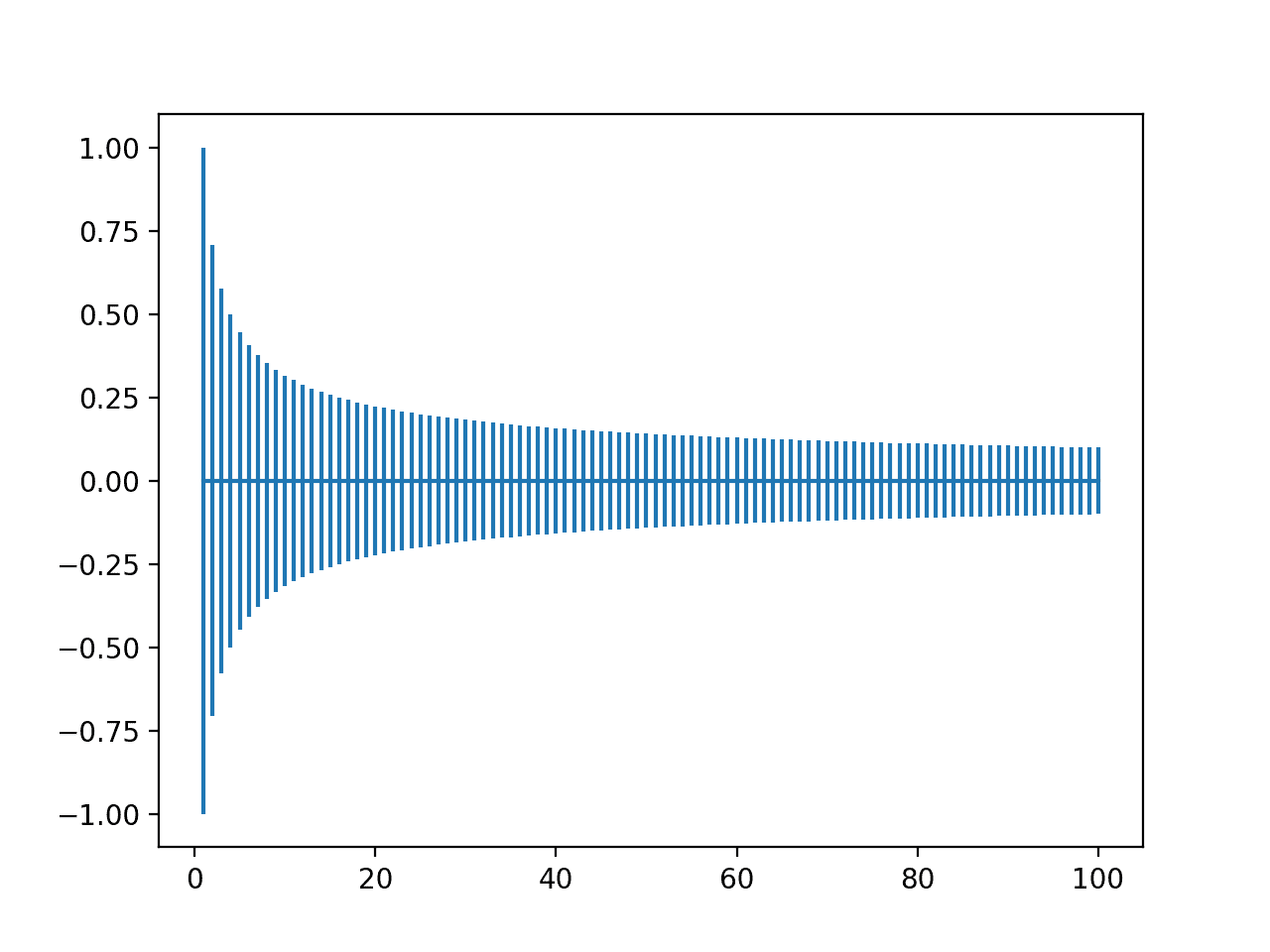
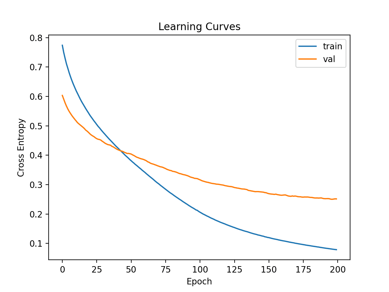
Line plots of the MSE on the train and test sets are then created.
We can see that the model has a good fit and converges nicely. The configuration of the model is a good starting point.
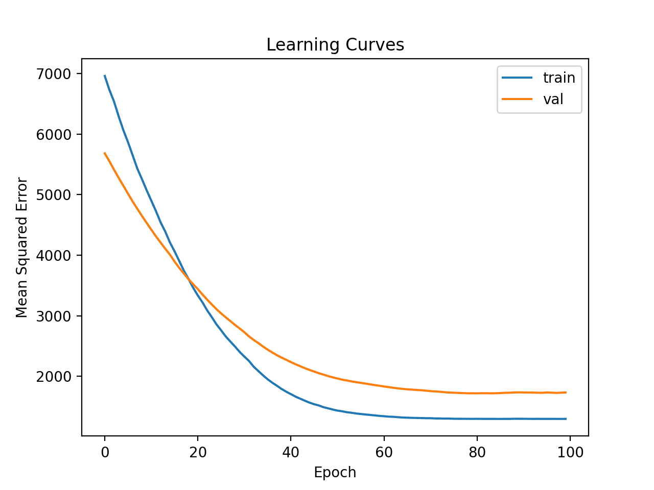
Learning Curves of Simple MLP on Auto Insurance Dataset
The learning dynamics are good so far, and the MAE is a rough estimate and should not be relied upon.
We can probably increase the capacity of the model a little and expect similar learning dynamics. For example, we can add a second hidden layer with eight nodes (chosen arbitrarily) and double the number of training epochs to 200.
...
# define model
model = Sequential()
model.add(Dense(10, activation='relu', kernel_initializer='he_normal', input_shape=(n_features,)))
model.add(Dense(8, activation='relu', kernel_initializer='he_normal'))
model.add(Dense(1))
# compile the model
model.compile(optimizer='adam', loss='mse')
# fit the model
history = model.fit(X_train, y_train, epochs=200, batch_size=8, verbose=0, validation_data=(X_test,y_test))
The complete example is listed below.
# fit a deeper mlp model and review learning curves
from pandas import read_csv
from sklearn.model_selection import train_test_split
from sklearn.metrics import mean_absolute_error
from tensorflow.keras import Sequential
from tensorflow.keras.layers import Dense
from matplotlib import pyplot
# load the dataset
path = 'https://raw.githubusercontent.com/jbrownlee/Datasets/master/auto-insurance.csv'
df = read_csv(path, header=None)
# split into input and output columns
X, y = df.values[:, :-1], df.values[:, -1]
# split into train and test datasets
X_train, X_test, y_train, y_test = train_test_split(X, y, test_size=0.33)
# determine the number of input features
n_features = X.shape[1]
# define model
model = Sequential()
model.add(Dense(10, activation='relu', kernel_initializer='he_normal', input_shape=(n_features,)))
model.add(Dense(8, activation='relu', kernel_initializer='he_normal'))
model.add(Dense(1))
# compile the model
model.compile(optimizer='adam', loss='mse')
# fit the model
history = model.fit(X_train, y_train, epochs=200, batch_size=8, verbose=0, validation_data=(X_test,y_test))
# predict test set
yhat = model.predict(X_test)
# evaluate predictions
score = mean_absolute_error(y_test, yhat)
print('MAE: %.3f' % score)
# plot learning curves
pyplot.title('Learning Curves')
pyplot.xlabel('Epoch')
pyplot.ylabel('Mean Squared Error')
pyplot.plot(history.history['loss'], label='train')
pyplot.plot(history.history['val_loss'], label='val')
pyplot.legend()
pyplot.show()
Running the example first fits the model on the training dataset, then reports the MAE on the test dataset.
Note: Your results may vary given the stochastic nature of the algorithm or evaluation procedure, or differences in numerical precision. Consider running the example a few times and compare the average outcome.
In this case, we can see a slight improvement in MAE to about 27.9, although the high variance of the train/test split means that this evaluation is not reliable.
MAE: 27.939
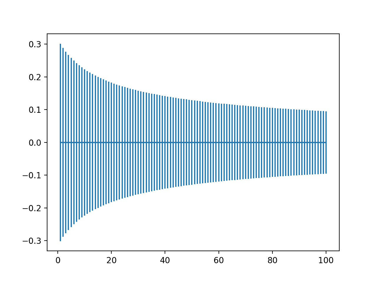
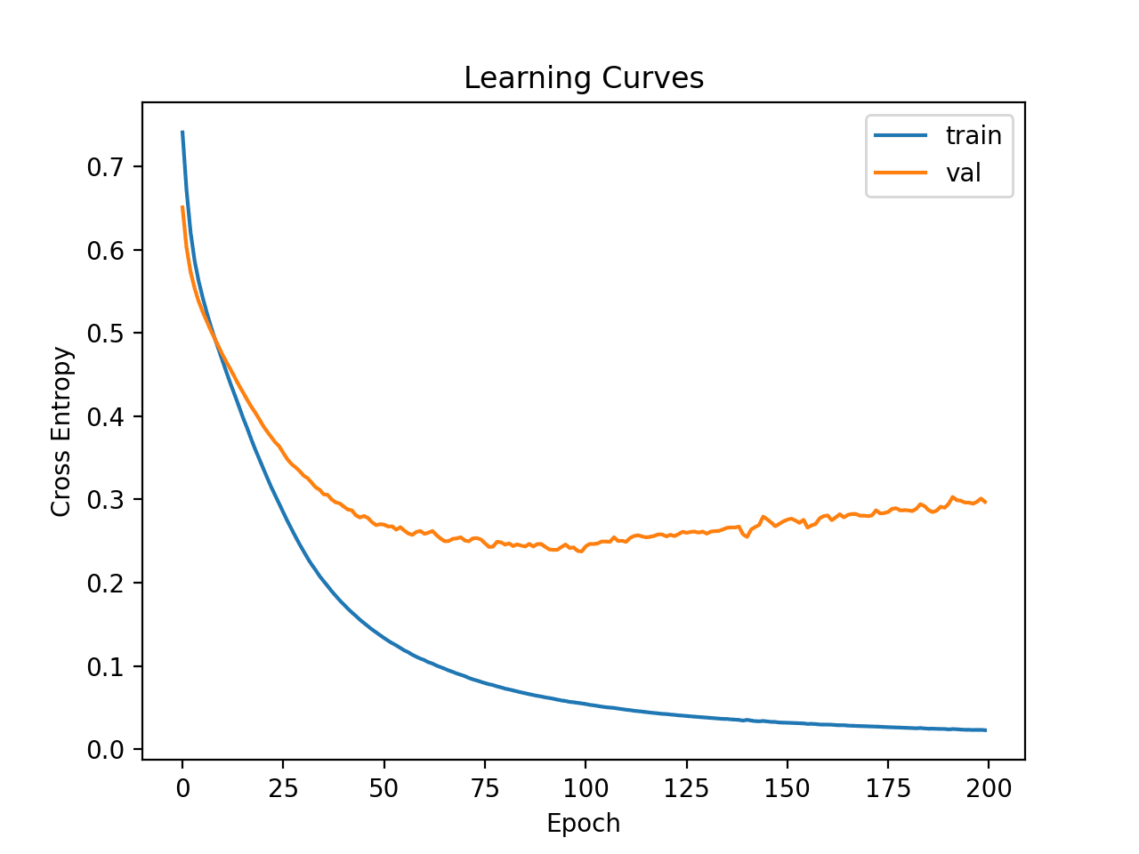
Learning curves for the MSE train and test sets are then plotted. We can see that, as expected, the model achieves a good fit and convergences within a reasonable number of iterations.
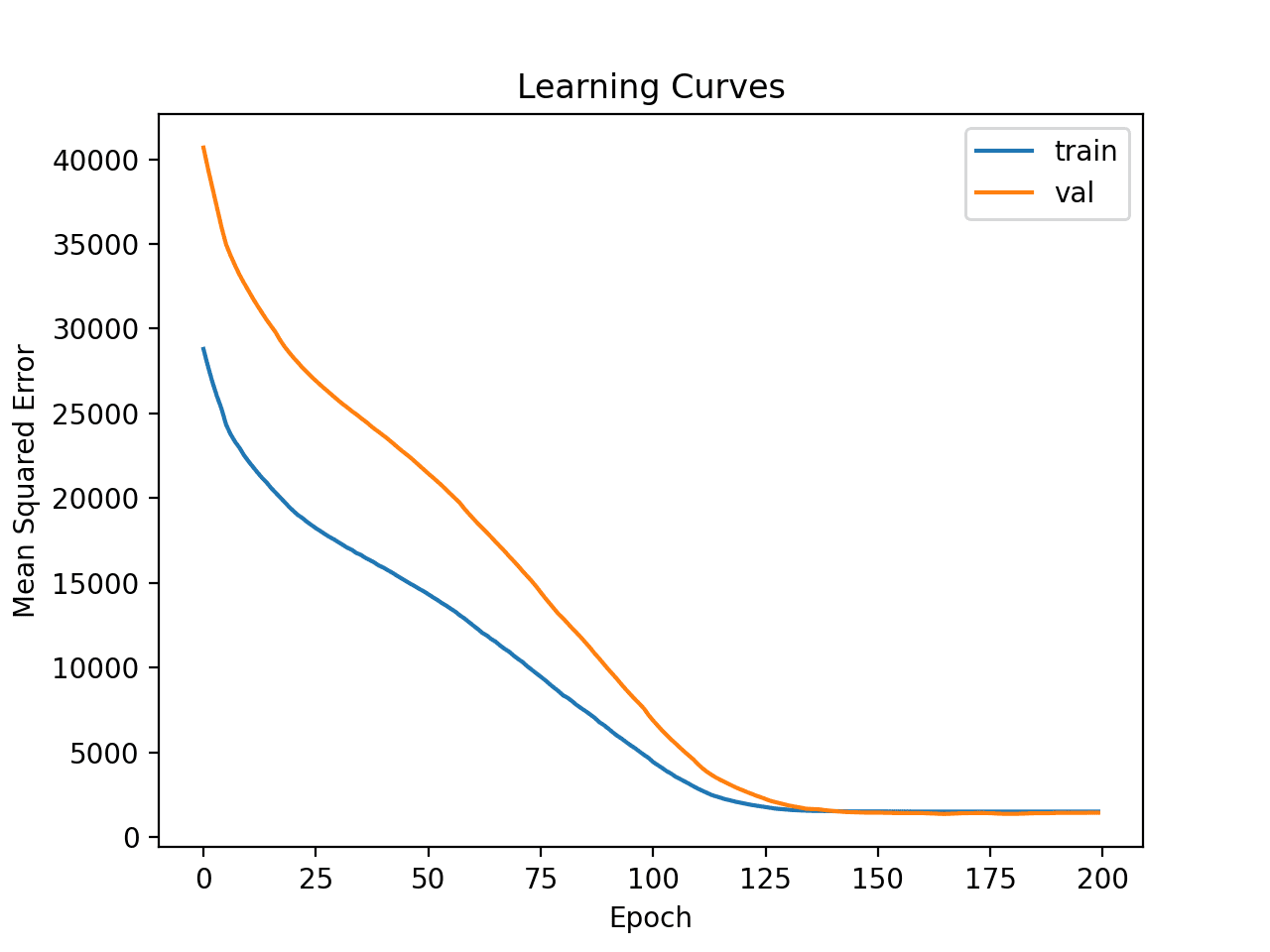
Learning Curves of Deeper MLP on Auto Insurance Dataset
Finally, we can try transforming the data and see how this impacts the learning dynamics.
In this case, we will use a power transform to make the data distribution less skewed. This will also automatically standardize the variables so that they have a mean of zero and a standard deviation of one — a good practice when modeling with a neural network.
First, we must ensure that the target variable is a two-dimensional array.
...
# ensure that the target variable is a 2d array
y_train, y_test = y_train.reshape((len(y_train),1)), y_test.reshape((len(y_test),1))
Next, we can apply a PowerTransformer to the input and target variables.
This can be achieved by first fitting the transform on the training data, then transforming the train and test sets.
This process is applied separately for the input and output variables to avoid data leakage.
...
# power transform input data
pt1 = PowerTransformer()
pt1.fit(X_train)
X_train = pt1.transform(X_train)
X_test = pt1.transform(X_test)
# power transform output data
pt2 = PowerTransformer()
pt2.fit(y_train)
y_train = pt2.transform(y_train)
y_test = pt2.transform(y_test)
The data is then used to fit the model.
The transform can then be inverted on the predictions made by the model and the expected target values from the test set and we can calculate the MAE in the correct scale as before.
...
# inverse transforms on target variable
y_test = pt2.inverse_transform(y_test)
yhat = pt2.inverse_transform(yhat)
Tying this together, the complete example of fitting and evaluating an MLP with transformed data and creating learning curves of the model is listed below.
# fit a mlp model with data transforms and review learning curves
from pandas import read_csv
from sklearn.model_selection import train_test_split
from sklearn.metrics import mean_absolute_error
from sklearn.preprocessing import PowerTransformer
from tensorflow.keras import Sequential
from tensorflow.keras.layers import Dense
from matplotlib import pyplot
# load the dataset
path = 'https://raw.githubusercontent.com/jbrownlee/Datasets/master/auto-insurance.csv'
df = read_csv(path, header=None)
# split into input and output columns
X, y = df.values[:, :-1], df.values[:, -1]
# split into train and test datasets
X_train, X_test, y_train, y_test = train_test_split(X, y, test_size=0.33)
# ensure that the target variable is a 2d array
y_train, y_test = y_train.reshape((len(y_train),1)), y_test.reshape((len(y_test),1))
# power transform input data
pt1 = PowerTransformer()
pt1.fit(X_train)
X_train = pt1.transform(X_train)
X_test = pt1.transform(X_test)
# power transform output data
pt2 = PowerTransformer()
pt2.fit(y_train)
y_train = pt2.transform(y_train)
y_test = pt2.transform(y_test)
# determine the number of input features
n_features = X.shape[1]
# define model
model = Sequential()
model.add(Dense(10, activation='relu', kernel_initializer='he_normal', input_shape=(n_features,)))
model.add(Dense(8, activation='relu', kernel_initializer='he_normal'))
model.add(Dense(1))
# compile the model
model.compile(optimizer='adam', loss='mse')
# fit the model
history = model.fit(X_train, y_train, epochs=200, batch_size=8, verbose=0, validation_data=(X_test,y_test))
# predict test set
yhat = model.predict(X_test)
# inverse transforms on target variable
y_test = pt2.inverse_transform(y_test)
yhat = pt2.inverse_transform(yhat)
# evaluate predictions
score = mean_absolute_error(y_test, yhat)
print('MAE: %.3f' % score)
# plot learning curves
pyplot.title('Learning Curves')
pyplot.xlabel('Epoch')
pyplot.ylabel('Mean Squared Error')
pyplot.plot(history.history['loss'], label='train')
pyplot.plot(history.history['val_loss'], label='val')
pyplot.legend()
pyplot.show()
Running the example first fits the model on the training dataset, then reports the MAE on the test dataset.
Note: Your results may vary given the stochastic nature of the algorithm or evaluation procedure, or differences in numerical precision. Consider running the example a few times and compare the average outcome.
In this case, the model achieves a reasonable MAE score, although worse than the performance reported previously. We will ignore model performance for now.
MAE: 34.320
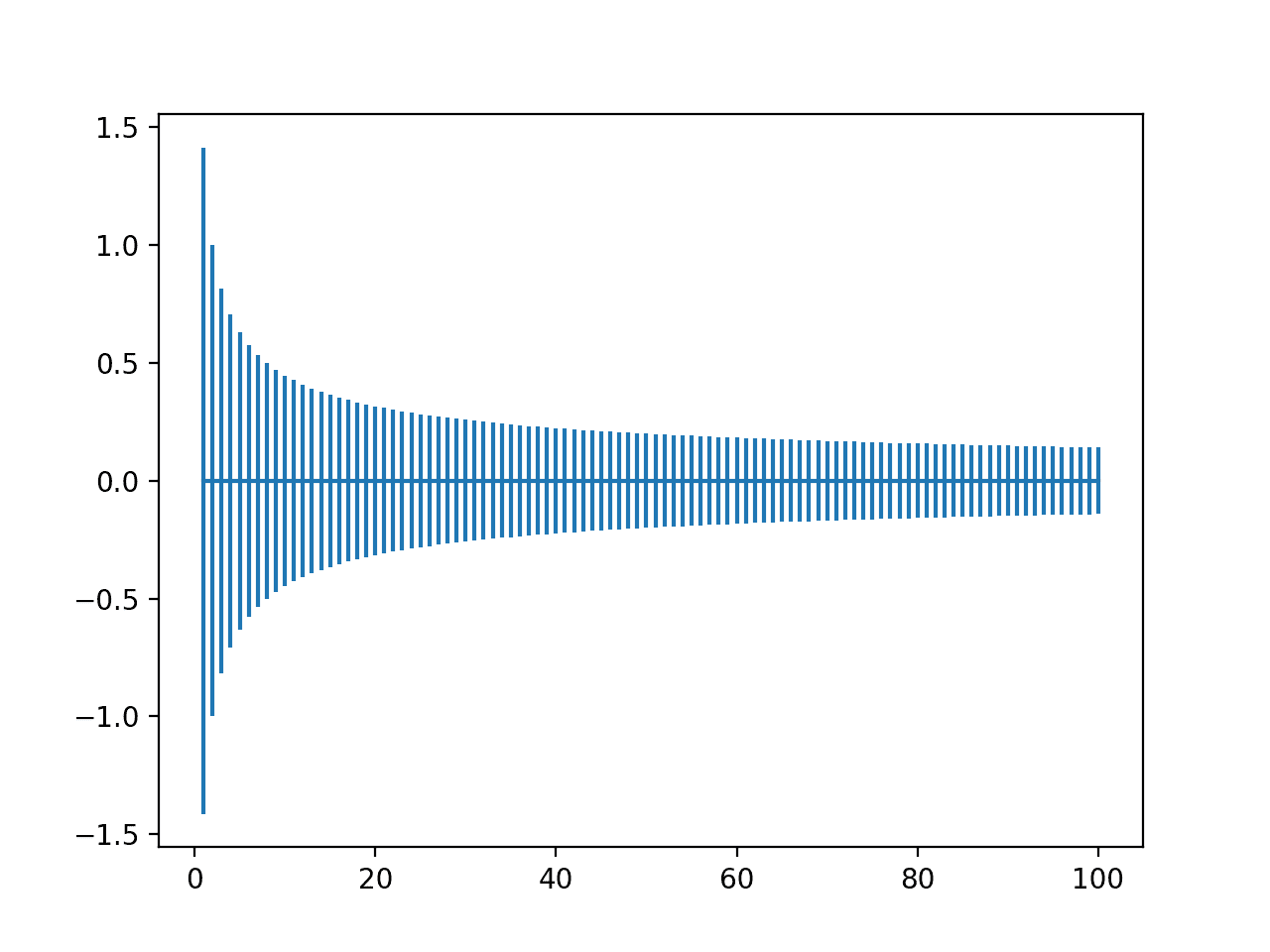
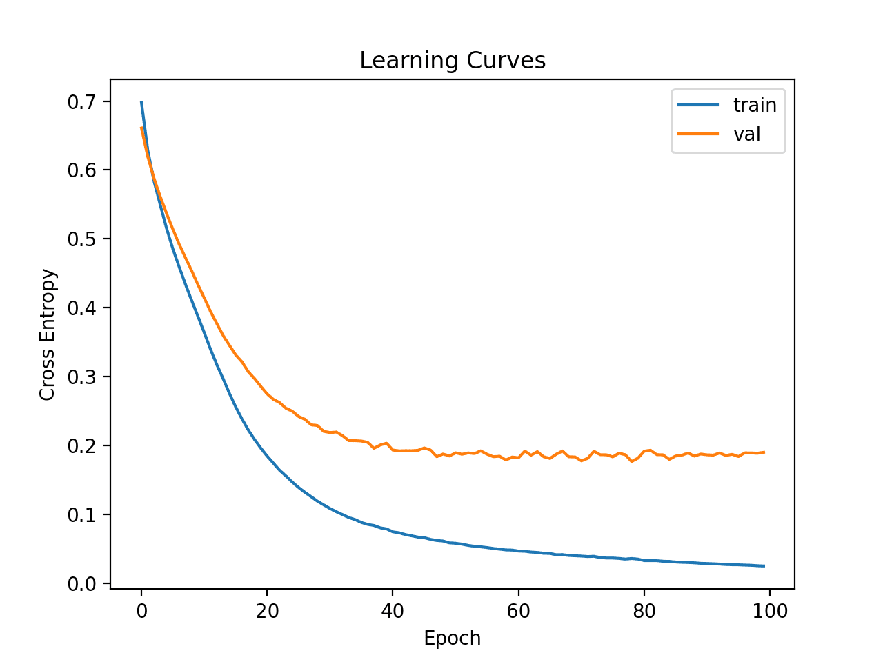
Line plots of the learning curves are created showing that the model achieved a reasonable fit and had more than enough time to converge.
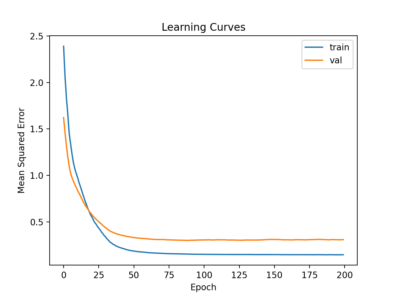
Learning Curves of Deeper MLP With Data Transforms on the Auto Insurance Dataset
Now that we have some idea of the learning dynamics for simple MLP models with and without data transforms, we can look at evaluating the performance of the models as well as tuning the configuration of the models.
Evaluating and Tuning MLP Models
The k-fold cross-validation procedure can provide a more reliable estimate of MLP performance, although it can be very slow.
This is because k models must be fit and evaluated. This is not a problem when the dataset size is small, such as the auto insurance dataset.
We can use the KFold class to create the splits and enumerate each fold manually, fit the model, evaluate it, and then report the mean of the evaluation scores at the end of the procedure.
# prepare cross validation
kfold = KFold(10)
# enumerate splits
scores = list()
for train_ix, test_ix in kfold.split(X, y):
	# fit and evaluate the model...
	...
...
# summarize all scores
print('Mean MAE: %.3f (%.3f)' % (mean(scores), std(scores)))
We can use this framework to develop a reliable estimate of MLP model performance with a range of different data preparations, model architectures, and learning configurations.
It is important that we first developed an understanding of the learning dynamics of the model on the dataset in the previous section before using k-fold cross-validation to estimate the performance. If we started to tune the model directly, we might get good results, but if not, we might have no idea of why, e.g. that the model was over or under fitting.
If we make large changes to the model again, it is a good idea to go back and confirm that model is converging appropriately.
The complete example of this framework to evaluate the base MLP model from the previous section is listed below.
# k-fold cross-validation of base model for the auto insurance regression dataset
from numpy import mean
from numpy import std
from pandas import read_csv
from sklearn.model_selection import KFold
from sklearn.metrics import mean_absolute_error
from tensorflow.keras import Sequential
from tensorflow.keras.layers import Dense
from matplotlib import pyplot
# load the dataset
path = 'https://raw.githubusercontent.com/jbrownlee/Datasets/master/auto-insurance.csv'
df = read_csv(path, header=None)
# split into input and output columns
X, y = df.values[:, :-1], df.values[:, -1]
# prepare cross validation
kfold = KFold(10)
# enumerate splits
scores = list()
for train_ix, test_ix in kfold.split(X, y):
	# split data
	X_train, X_test, y_train, y_test = X[train_ix], X[test_ix], y[train_ix], y[test_ix]
	# determine the number of input features
	n_features = X.shape[1]
	# define model
	model = Sequential()
	model.add(Dense(10, activation='relu', kernel_initializer='he_normal', input_shape=(n_features,)))
	model.add(Dense(1))
	# compile the model
	model.compile(optimizer='adam', loss='mse')
	# fit the model
	model.fit(X_train, y_train, epochs=100, batch_size=8, verbose=0)
	# predict test set
	yhat = model.predict(X_test)
	# evaluate predictions
	score = mean_absolute_error(y_test, yhat)
	print('>%.3f' % score)
	scores.append(score)
# summarize all scores
print('Mean MAE: %.3f (%.3f)' % (mean(scores), std(scores)))
Running the example reports the model performance each iteration of the evaluation procedure and reports the mean and standard deviation of the MAE at the end of the run.
Note: Your results may vary given the stochastic nature of the algorithm or evaluation procedure, or differences in numerical precision. Consider running the example a few times and compare the average outcome.
In this case, we can see that the MLP model achieved a MAE of about 38.913.
We will use this result as our baseline to see if we can achieve better performance.
>27.314
>69.577
>20.891
>14.810
>13.412
>69.540
>25.612
>49.508
>35.769
>62.696
Mean MAE: 38.913 (21.056)
First, let’s try evaluating a deeper model on the raw dataset to see if it performs any better than a baseline model.
...
# define model
model = Sequential()
model.add(Dense(10, activation='relu', kernel_initializer='he_normal', input_shape=(n_features,)))
model.add(Dense(8, activation='relu', kernel_initializer='he_normal'))
model.add(Dense(1))
# compile the model
model.compile(optimizer='adam', loss='mse')
# fit the model
model.fit(X_train, y_train, epochs=200, batch_size=8, verbose=0)
The complete example is listed below.
# k-fold cross-validation of deeper model for the auto insurance regression dataset
from numpy import mean
from numpy import std
from pandas import read_csv
from sklearn.model_selection import KFold
from sklearn.metrics import mean_absolute_error
from tensorflow.keras import Sequential
from tensorflow.keras.layers import Dense
from matplotlib import pyplot
# load the dataset
path = 'https://raw.githubusercontent.com/jbrownlee/Datasets/master/auto-insurance.csv'
df = read_csv(path, header=None)
# split into input and output columns
X, y = df.values[:, :-1], df.values[:, -1]
# prepare cross validation
kfold = KFold(10)
# enumerate splits
scores = list()
for train_ix, test_ix in kfold.split(X, y):
	# split data
	X_train, X_test, y_train, y_test = X[train_ix], X[test_ix], y[train_ix], y[test_ix]
	# determine the number of input features
	n_features = X.shape[1]
	# define model
	model = Sequential()
	model.add(Dense(10, activation='relu', kernel_initializer='he_normal', input_shape=(n_features,)))
	model.add(Dense(8, activation='relu', kernel_initializer='he_normal'))
	model.add(Dense(1))
	# compile the model
	model.compile(optimizer='adam', loss='mse')
	# fit the model
	model.fit(X_train, y_train, epochs=200, batch_size=8, verbose=0)
	# predict test set
	yhat = model.predict(X_test)
	# evaluate predictions
	score = mean_absolute_error(y_test, yhat)
	print('>%.3f' % score)
	scores.append(score)
# summarize all scores
print('Mean MAE: %.3f (%.3f)' % (mean(scores), std(scores)))
Running reports the mean and standard deviation of the MAE at the end of the run.
Note: Your results may vary given the stochastic nature of the algorithm or evaluation procedure, or differences in numerical precision. Consider running the example a few times and compare the average outcome.
In this case, we can see that the MLP model achieved a MAE of about 35.384, which is slightly better than the baseline model that achieved an MAE of about 38.913.
Mean MAE: 35.384 (14.951)
Next, let’s try using the same model with a power transform for the input and target variables as we did in the previous section.
The complete example is listed below.
# k-fold cross-validation of deeper model with data transforms
from numpy import mean
from numpy import std
from pandas import read_csv
from sklearn.model_selection import KFold
from sklearn.metrics import mean_absolute_error
from sklearn.preprocessing import PowerTransformer
from tensorflow.keras import Sequential
from tensorflow.keras.layers import Dense
from matplotlib import pyplot
# load the dataset
path = 'https://raw.githubusercontent.com/jbrownlee/Datasets/master/auto-insurance.csv'
df = read_csv(path, header=None)
# split into input and output columns
X, y = df.values[:, :-1], df.values[:, -1]
# prepare cross validation
kfold = KFold(10)
# enumerate splits
scores = list()
for train_ix, test_ix in kfold.split(X, y):
	# split data
	X_train, X_test, y_train, y_test = X[train_ix], X[test_ix], y[train_ix], y[test_ix]
	# ensure target is a 2d array
	y_train, y_test = y_train.reshape((len(y_train),1)), y_test.reshape((len(y_test),1))
	# prepare input data
	pt1 = PowerTransformer()
	pt1.fit(X_train)
	X_train = pt1.transform(X_train)
	X_test = pt1.transform(X_test)
	# prepare target
	pt2 = PowerTransformer()
	pt2.fit(y_train)
	y_train = pt2.transform(y_train)
	y_test = pt2.transform(y_test)
	# determine the number of input features
	n_features = X.shape[1]
	# define model
	model = Sequential()
	model.add(Dense(10, activation='relu', kernel_initializer='he_normal', input_shape=(n_features,)))
	model.add(Dense(8, activation='relu', kernel_initializer='he_normal'))
	model.add(Dense(1))
	# compile the model
	model.compile(optimizer='adam', loss='mse')
	# fit the model
	model.fit(X_train, y_train, epochs=200, batch_size=8, verbose=0)
	# predict test set
	yhat = model.predict(X_test)
	# inverse transforms
	y_test = pt2.inverse_transform(y_test)
	yhat = pt2.inverse_transform(yhat)
	# evaluate predictions
	score = mean_absolute_error(y_test, yhat)
	print('>%.3f' % score)
	scores.append(score)
# summarize all scores
print('Mean MAE: %.3f (%.3f)' % (mean(scores), std(scores)))
Running reports the mean and standard deviation of the MAE at the end of the run.
Note: Your results may vary given the stochastic nature of the algorithm or evaluation procedure, or differences in numerical precision. Consider running the example a few times and compare the average outcome.
In this case, we can see that the MLP model achieved a MAE of about 37.371, which is better than the baseline model, but not better than the deeper baseline model.
Perhaps this transform is not as helpful as we initially thought.
Mean MAE: 37.371 (29.326)
An alternate transform is to normalize the input and target variables.
This means to scale the values of each variable to the range [0, 1]. We can achieve this using the MinMaxScaler; for example:
...
# prepare input data
pt1 = MinMaxScaler()
pt1.fit(X_train)
X_train = pt1.transform(X_train)
X_test = pt1.transform(X_test)
# prepare target
pt2 = MinMaxScaler()
pt2.fit(y_train)
y_train = pt2.transform(y_train)
y_test = pt2.transform(y_test)
Tying this together, the complete example of evaluating the deeper MLP with data normalization is listed below.
# k-fold cross-validation of deeper model with normalization transforms
from numpy import mean
from numpy import std
from pandas import read_csv
from sklearn.model_selection import KFold
from sklearn.metrics import mean_absolute_error
from sklearn.preprocessing import MinMaxScaler
from tensorflow.keras import Sequential
from tensorflow.keras.layers import Dense
from matplotlib import pyplot
# load the dataset
path = 'https://raw.githubusercontent.com/jbrownlee/Datasets/master/auto-insurance.csv'
df = read_csv(path, header=None)
# split into input and output columns
X, y = df.values[:, :-1], df.values[:, -1]
# prepare cross validation
kfold = KFold(10)
# enumerate splits
scores = list()
for train_ix, test_ix in kfold.split(X, y):
	# split data
	X_train, X_test, y_train, y_test = X[train_ix], X[test_ix], y[train_ix], y[test_ix]
	# ensure target is a 2d array
	y_train, y_test = y_train.reshape((len(y_train),1)), y_test.reshape((len(y_test),1))
	# prepare input data
	pt1 = MinMaxScaler()
	pt1.fit(X_train)
	X_train = pt1.transform(X_train)
	X_test = pt1.transform(X_test)
	# prepare target
	pt2 = MinMaxScaler()
	pt2.fit(y_train)
	y_train = pt2.transform(y_train)
	y_test = pt2.transform(y_test)
	# determine the number of input features
	n_features = X.shape[1]
	# define model
	model = Sequential()
	model.add(Dense(10, activation='relu', kernel_initializer='he_normal', input_shape=(n_features,)))
	model.add(Dense(8, activation='relu', kernel_initializer='he_normal'))
	model.add(Dense(1))
	# compile the model
	model.compile(optimizer='adam', loss='mse')
	# fit the model
	model.fit(X_train, y_train, epochs=200, batch_size=8, verbose=0)
	# predict test set
	yhat = model.predict(X_test)
	# inverse transforms
	y_test = pt2.inverse_transform(y_test)
	yhat = pt2.inverse_transform(yhat)
	# evaluate predictions
	score = mean_absolute_error(y_test, yhat)
	print('>%.3f' % score)
	scores.append(score)
# summarize all scores
print('Mean MAE: %.3f (%.3f)' % (mean(scores), std(scores)))
Running reports the mean and standard deviation of the MAE at the end of the run.
Note: Your results may vary given the stochastic nature of the algorithm or evaluation procedure, or differences in numerical precision. Consider running the example a few times and compare the average outcome.
In this case, we can see that the MLP model achieved a MAE of about 30.388, which is better than any other configuration we have tried so far.
Mean MAE: 30.388 (14.258)
We could continue to test alternate configurations to the model architecture (more or fewer nodes or layers), learning hyperparameters (more or fewer batches), and data transforms.
I leave this as an exercise; let me know what you discover. Can you get better results?
Post your results in the comments below, I’d love to see what you get.
Next, let’s look at how we might fit a final model and use it to make predictions.
Final Model and Make Predictions
Once we choose a model configuration, we can train a final model on all available data and use it to make predictions on new data.
In this case, we will use the deeper model with data normalization as our final model.
This means if we wanted to save the model to file, we would have to save the model itself (for making predictions), the transform for input data (for new input data), and the transform for target variable (for new predictions).
We can prepare the data and fit the model as before, although on the entire dataset instead of a training subset of the dataset.
...
# split into input and output columns
X, y = df.values[:, :-1], df.values[:, -1]
# ensure target is a 2d array
y = y.reshape((len(y),1))
# prepare input data
pt1 = MinMaxScaler()
pt1.fit(X)
X = pt1.transform(X)
# prepare target
pt2 = MinMaxScaler()
pt2.fit(y)
y = pt2.transform(y)
# determine the number of input features
n_features = X.shape[1]
# define model
model = Sequential()
model.add(Dense(10, activation='relu', kernel_initializer='he_normal', input_shape=(n_features,)))
model.add(Dense(8, activation='relu', kernel_initializer='he_normal'))
model.add(Dense(1))
# compile the model
model.compile(optimizer='adam', loss='mse')
We can then use this model to make predictions on new data.
First, we can define a row of new data, which is just one variable for this dataset.
...
# define a row of new data
row = [13]
We can then transform this new data ready to be used as input to the model.
...
# transform the input data
X_new = pt1.transform([row])
We can then make a prediction.
...
# make prediction
yhat = model.predict(X_new)
Then invert the transform on the prediction so we can use or interpret the result in the correct scale.
...
# invert transform on prediction
yhat = pt2.inverse_transform(yhat)
And in this case, we will simply report the prediction.
...
# report prediction
print('f(%s) = %.3f' % (row, yhat[0]))
Tying this all together, the complete example of fitting a final model for the auto insurance dataset and using it to make a prediction on new data is listed below.
# fit a final model and make predictions on new data.
from pandas import read_csv
from sklearn.model_selection import KFold
from sklearn.metrics import mean_absolute_error
from sklearn.preprocessing import MinMaxScaler
from tensorflow.keras import Sequential
from tensorflow.keras.layers import Dense
# load the dataset
path = 'https://raw.githubusercontent.com/jbrownlee/Datasets/master/auto-insurance.csv'
df = read_csv(path, header=None)
# split into input and output columns
X, y = df.values[:, :-1], df.values[:, -1]
# ensure target is a 2d array
y = y.reshape((len(y),1))
# prepare input data
pt1 = MinMaxScaler()
pt1.fit(X)
X = pt1.transform(X)
# prepare target
pt2 = MinMaxScaler()
pt2.fit(y)
y = pt2.transform(y)
# determine the number of input features
n_features = X.shape[1]
# define model
model = Sequential()
model.add(Dense(10, activation='relu', kernel_initializer='he_normal', input_shape=(n_features,)))
model.add(Dense(8, activation='relu', kernel_initializer='he_normal'))
model.add(Dense(1))
# compile the model
model.compile(optimizer='adam', loss='mse')
# fit the model
model.fit(X, y, epochs=200, batch_size=8, verbose=0)
# define a row of new data
row = [13]
# transform the input data
X_new = pt1.transform([row])
# make prediction
yhat = model.predict(X_new)
# invert transform on prediction
yhat = pt2.inverse_transform(yhat)
# report prediction
print('f(%s) = %.3f' % (row, yhat[0]))
Running the example fits the model on the entire dataset and makes a prediction for a single row of new data.
Note: Your results may vary given the stochastic nature of the algorithm or evaluation procedure, or differences in numerical precision. Consider running the example a few times and compare the average outcome.
In this case, we can see that an input of 13 results in an output of 62 (thousand Swedish Krona).
f([13]) = 62.595
Further Reading
This section provides more resources on the topic if you are looking to go deeper.
Tutorials
- Best Results for Standard Machine Learning Datasets
- TensorFlow 2 Tutorial: Get Started in Deep Learning With tf.keras
- A Gentle Introduction to k-fold Cross-Validation
Summary
In this tutorial, you discovered how to develop a Multilayer Perceptron neural network model for the Swedish car insurance regression dataset.
Specifically, you learned:
- How to load and summarize the Swedish car insurance dataset and use the results to suggest data preparations and model configurations to use.
- How to explore the learning dynamics of simple MLP models and data transforms on the dataset.
- How to develop robust estimates of model performance, tune model performance and make predictions on new data.
Do you have any questions?
Ask your questions in the comments below and I will do my best to answer.
The post How to Develop a Neural Net for Predicting Car Insurance Payout appeared first on Machine Learning Mastery.