Machine learning algorithms have hyperparameters that allow you to tailor the behavior of the algorithm to your specific dataset.

Hyperparameters are different from parameters, which are the internal coefficients or weights for a model found by the learning algorithm. Unlike parameters, hyperparameters are specified by the practitioner when configuring the model.

Typically, it is challenging to know what values to use for the hyperparameters of a given algorithm on a given dataset, therefore it is common to use random or grid search strategies for different hyperparameter values.

The more hyperparameters of an algorithm that you need to tune, the slower the tuning process. Therefore, it is desirable to select a minimum subset of model hyperparameters to search or tune.

Not all model hyperparameters are equally important. Some hyperparameters have an outsized effect on the behavior, and in turn, the performance of a machine learning algorithm.

As a machine learning practitioner, you must know which hyperparameters to focus on to get a good result quickly.

In this tutorial, you will discover those hyperparameters that are most important for some of the top machine learning algorithms.

Let’s get started.

Hyperparameters for Classification Machine Learning Algorithms
Photo by shuttermonkey, some rights reserved.

Classification Algorithms Overview

We will take a closer look at the important hyperparameters of the top machine learning algorithms that you may use for classification.

We will look at the hyperparameters you need to focus on and suggested values to try when tuning the model on your dataset.

The suggestions are based both on advice from textbooks on the algorithms and practical advice suggested by practitioners, as well as a little of my own experience.

The seven classification algorithms we will look at are as follows:

1. Logistic Regression
2. Ridge Classifier
3. K-Nearest Neighbors (KNN)
4. Support Vector Machine (SVM)
5. Bagged Decision Trees (Bagging)
6. Random Forest
7. Stochastic Gradient Boosting

We will consider these algorithms in the context of their scikit-learn implementation (Python); nevertheless, you can use the same hyperparameter suggestions with other platforms, such as Weka and R.

A small grid searching example is also given for each algorithm that you can use as a starting point for your own classification predictive modeling project.

Note: if you have had success with different hyperparameter values or even different hyperparameters than those suggested in this tutorial, let me know in the comments below. I’d love to hear about it.

Let’s dive in.

Logistic Regression

Logistic regression does not really have any critical hyperparameters to tune.

Sometimes, you can see useful differences in performance or convergence with different solvers (solver).

• solver in [‘newton-cg’, ‘lbfgs’, ‘liblinear’, ‘sag’, ‘saga’]

Regularization (penalty) can sometimes be helpful.

• penalty in [‘none’, ‘l1’, ‘l2’, ‘elasticnet’]

Note: not all solvers support all regularization terms.

The C parameter controls the penality strength, which can also be effective.

• C in [100, 10, 1.0, 0.1, 0.01]

For the full list of hyperparameters, see:

• sklearn.linear_model.LogisticRegression API.

The example below demonstrates grid searching the key hyperparameters for LogisticRegression on a synthetic binary classification dataset.

Some combinations were omitted to cut back on the warnings/errors.

# example of grid searching key hyperparametres for logistic regression
from sklearn.datasets.samples_generator import make_blobs
from sklearn.model_selection import RepeatedStratifiedKFold
from sklearn.model_selection import GridSearchCV
from sklearn.linear_model import LogisticRegression
# define dataset
X, y = make_blobs(n_samples=1000, centers=2, n_features=100, cluster_std=20)
# define models and parameters
model = LogisticRegression()
solvers = ['newton-cg', 'lbfgs', 'liblinear']
penalty = ['l2']
c_values = [100, 10, 1.0, 0.1, 0.01]
# define grid search
grid = dict(solver=solvers,penalty=penalty,C=c_values)
cv = RepeatedStratifiedKFold(n_splits=10, n_repeats=3, random_state=1)
grid_search = GridSearchCV(estimator=model, param_grid=grid, n_jobs=-1, cv=cv, scoring='accuracy',error_score=0)
grid_result = grid_search.fit(X, y)
# summarize results
print("Best: %f using %s" % (grid_result.best_score_, grid_result.best_params_))
means = grid_result.cv_results_['mean_test_score']
stds = grid_result.cv_results_['std_test_score']
params = grid_result.cv_results_['params']
for mean, stdev, param in zip(means, stds, params):
    print("%f (%f) with: %r" % (mean, stdev, param))

Running the example prints the best result as well as the results from all combinations evaluated.

Best: 0.945333 using {'C': 0.01, 'penalty': 'l2', 'solver': 'liblinear'}
0.936333 (0.016829) with: {'C': 100, 'penalty': 'l2', 'solver': 'newton-cg'}
0.937667 (0.017259) with: {'C': 100, 'penalty': 'l2', 'solver': 'lbfgs'}
0.938667 (0.015861) with: {'C': 100, 'penalty': 'l2', 'solver': 'liblinear'}
0.936333 (0.017413) with: {'C': 10, 'penalty': 'l2', 'solver': 'newton-cg'}
0.938333 (0.017904) with: {'C': 10, 'penalty': 'l2', 'solver': 'lbfgs'}
0.939000 (0.016401) with: {'C': 10, 'penalty': 'l2', 'solver': 'liblinear'}
0.937333 (0.017114) with: {'C': 1.0, 'penalty': 'l2', 'solver': 'newton-cg'}
0.939000 (0.017195) with: {'C': 1.0, 'penalty': 'l2', 'solver': 'lbfgs'}
0.939000 (0.015780) with: {'C': 1.0, 'penalty': 'l2', 'solver': 'liblinear'}
0.940000 (0.015706) with: {'C': 0.1, 'penalty': 'l2', 'solver': 'newton-cg'}
0.940333 (0.014941) with: {'C': 0.1, 'penalty': 'l2', 'solver': 'lbfgs'}
0.941000 (0.017000) with: {'C': 0.1, 'penalty': 'l2', 'solver': 'liblinear'}
0.943000 (0.016763) with: {'C': 0.01, 'penalty': 'l2', 'solver': 'newton-cg'}
0.943000 (0.016763) with: {'C': 0.01, 'penalty': 'l2', 'solver': 'lbfgs'}
0.945333 (0.017651) with: {'C': 0.01, 'penalty': 'l2', 'solver': 'liblinear'}

Ridge Classifier

Ridge regression is a penalized linear regression model for predicting a numerical value.

Nevertheless, it can be very effective when applied to classification.

Perhaps the most important parameter to tune is the regularization strength (alpha). A good starting point might be values in the range [0.1 to 1.0]

• alpha in [0.1, 0.2, 0.3, 0.4, 0.5, 0.6, 0.7, 0.8, 0.9, 1.0]

For the full list of hyperparameters, see:

• sklearn.linear_model.RidgeClassifier API.

The example below demonstrates grid searching the key hyperparameters for RidgeClassifier on a synthetic binary classification dataset.

# example of grid searching key hyperparametres for ridge classifier
from sklearn.datasets.samples_generator import make_blobs
from sklearn.model_selection import RepeatedStratifiedKFold
from sklearn.model_selection import GridSearchCV
from sklearn.linear_model import RidgeClassifier
# define dataset
X, y = make_blobs(n_samples=1000, centers=2, n_features=100, cluster_std=20)
# define models and parameters
model = RidgeClassifier()
alpha = [0.1, 0.2, 0.3, 0.4, 0.5, 0.6, 0.7, 0.8, 0.9, 1.0]
# define grid search
grid = dict(alpha=alpha)
cv = RepeatedStratifiedKFold(n_splits=10, n_repeats=3, random_state=1)
grid_search = GridSearchCV(estimator=model, param_grid=grid, n_jobs=-1, cv=cv, scoring='accuracy',error_score=0)
grid_result = grid_search.fit(X, y)
# summarize results
print("Best: %f using %s" % (grid_result.best_score_, grid_result.best_params_))
means = grid_result.cv_results_['mean_test_score']
stds = grid_result.cv_results_['std_test_score']
params = grid_result.cv_results_['params']
for mean, stdev, param in zip(means, stds, params):
    print("%f (%f) with: %r" % (mean, stdev, param))

Running the example prints the best result as well as the results from all combinations evaluated.

Best: 0.974667 using {'alpha': 0.1}
0.974667 (0.014545) with: {'alpha': 0.1}
0.974667 (0.014545) with: {'alpha': 0.2}
0.974667 (0.014545) with: {'alpha': 0.3}
0.974667 (0.014545) with: {'alpha': 0.4}
0.974667 (0.014545) with: {'alpha': 0.5}
0.974667 (0.014545) with: {'alpha': 0.6}
0.974667 (0.014545) with: {'alpha': 0.7}
0.974667 (0.014545) with: {'alpha': 0.8}
0.974667 (0.014545) with: {'alpha': 0.9}
0.974667 (0.014545) with: {'alpha': 1.0}

K-Nearest Neighbors (KNN)

The most important hyperparameter for KNN is the number of neighbors (n_neighbors).

Test values between at least 1 and 21, perhaps just the odd numbers.

• n_neighbors in [1 to 21]

It may also be interesting to test different distance metrics (metric) for choosing the composition of the neighborhood.

• metric in [‘euclidean’, ‘manhattan’, ‘minkowski’]

For a fuller list see:

• sklearn.neighbors.DistanceMetric API

It may also be interesting to test the contribution of members of the neighborhood via different weightings (weights).

• weights in [‘uniform’, ‘distance’]

For the full list of hyperparameters, see:

• sklearn.neighbors.KNeighborsClassifier API.

The example below demonstrates grid searching the key hyperparameters for KNeighborsClassifier on a synthetic binary classification dataset.

# example of grid searching key hyperparametres for KNeighborsClassifier
from sklearn.datasets.samples_generator import make_blobs
from sklearn.model_selection import RepeatedStratifiedKFold
from sklearn.model_selection import GridSearchCV
from sklearn.neighbors import KNeighborsClassifier
# define dataset
X, y = make_blobs(n_samples=1000, centers=2, n_features=100, cluster_std=20)
# define models and parameters
model = KNeighborsClassifier()
n_neighbors = range(1, 21, 2)
weights = ['uniform', 'distance']
metric = ['euclidean', 'manhattan', 'minkowski']
# define grid search
grid = dict(n_neighbors=n_neighbors,weights=weights,metric=metric)
cv = RepeatedStratifiedKFold(n_splits=10, n_repeats=3, random_state=1)
grid_search = GridSearchCV(estimator=model, param_grid=grid, n_jobs=-1, cv=cv, scoring='accuracy',error_score=0)
grid_result = grid_search.fit(X, y)
# summarize results
print("Best: %f using %s" % (grid_result.best_score_, grid_result.best_params_))
means = grid_result.cv_results_['mean_test_score']
stds = grid_result.cv_results_['std_test_score']
params = grid_result.cv_results_['params']
for mean, stdev, param in zip(means, stds, params):
    print("%f (%f) with: %r" % (mean, stdev, param))

Running the example prints the best result as well as the results from all combinations evaluated.

Best: 0.937667 using {'metric': 'manhattan', 'n_neighbors': 13, 'weights': 'uniform'}
0.833667 (0.031674) with: {'metric': 'euclidean', 'n_neighbors': 1, 'weights': 'uniform'}
0.833667 (0.031674) with: {'metric': 'euclidean', 'n_neighbors': 1, 'weights': 'distance'}
0.895333 (0.030081) with: {'metric': 'euclidean', 'n_neighbors': 3, 'weights': 'uniform'}
0.895333 (0.030081) with: {'metric': 'euclidean', 'n_neighbors': 3, 'weights': 'distance'}
0.909000 (0.021810) with: {'metric': 'euclidean', 'n_neighbors': 5, 'weights': 'uniform'}
0.909000 (0.021810) with: {'metric': 'euclidean', 'n_neighbors': 5, 'weights': 'distance'}
0.925333 (0.020774) with: {'metric': 'euclidean', 'n_neighbors': 7, 'weights': 'uniform'}
0.925333 (0.020774) with: {'metric': 'euclidean', 'n_neighbors': 7, 'weights': 'distance'}
0.929000 (0.027368) with: {'metric': 'euclidean', 'n_neighbors': 9, 'weights': 'uniform'}
0.929000 (0.027368) with: {'metric': 'euclidean', 'n_neighbors': 9, 'weights': 'distance'}
...

Support Vector Machine (SVM)

The SVM algorithm, like gradient boosting, is very popular, very effective, and provides a large number of hyperparameters to tune.

Perhaps the first important parameter is the choice of kernel that will control the manner in which the input variables will be projected. There are many to choose from, but linear, polynomial, and RBF are the most common, perhaps just linear and RBF in practice.

• kernels in [‘linear’, ‘poly’, ‘rbf’, ‘sigmoid’]

If the polynomial kernel works out, then it is a good idea to dive into the degree hyperparameter.

Another critical parameter is the penalty (C) that can take on a range of values and has a dramatic effect on the shape of the resulting regions for each class. A log scale might be a good starting point.

• C in [100, 10, 1.0, 0.1, 0.001]

For the full list of hyperparameters, see:

• sklearn.svm.SVC API.

The example below demonstrates grid searching the key hyperparameters for SVC on a synthetic binary classification dataset.

# example of grid searching key hyperparametres for SVC
from sklearn.datasets.samples_generator import make_blobs
from sklearn.model_selection import RepeatedStratifiedKFold
from sklearn.model_selection import GridSearchCV
from sklearn.svm import SVC
# define dataset
X, y = make_blobs(n_samples=1000, centers=2, n_features=100, cluster_std=20)
# define model and parameters
model = SVC()
kernel = ['poly', 'rbf', 'sigmoid']
C = [50, 10, 1.0, 0.1, 0.01]
gamma = ['scale']
# define grid search
grid = dict(kernel=kernel,C=C,gamma=gamma)
cv = RepeatedStratifiedKFold(n_splits=10, n_repeats=3, random_state=1)
grid_search = GridSearchCV(estimator=model, param_grid=grid, n_jobs=-1, cv=cv, scoring='accuracy',error_score=0)
grid_result = grid_search.fit(X, y)
# summarize results
print("Best: %f using %s" % (grid_result.best_score_, grid_result.best_params_))
means = grid_result.cv_results_['mean_test_score']
stds = grid_result.cv_results_['std_test_score']
params = grid_result.cv_results_['params']
for mean, stdev, param in zip(means, stds, params):
    print("%f (%f) with: %r" % (mean, stdev, param))

Running the example prints the best result as well as the results from all combinations evaluated.

Best: 0.974333 using {'C': 1.0, 'gamma': 'scale', 'kernel': 'poly'}
0.973667 (0.012512) with: {'C': 50, 'gamma': 'scale', 'kernel': 'poly'}
0.970667 (0.018062) with: {'C': 50, 'gamma': 'scale', 'kernel': 'rbf'}
0.945333 (0.024594) with: {'C': 50, 'gamma': 'scale', 'kernel': 'sigmoid'}
0.973667 (0.012512) with: {'C': 10, 'gamma': 'scale', 'kernel': 'poly'}
0.970667 (0.018062) with: {'C': 10, 'gamma': 'scale', 'kernel': 'rbf'}
0.957000 (0.016763) with: {'C': 10, 'gamma': 'scale', 'kernel': 'sigmoid'}
0.974333 (0.012565) with: {'C': 1.0, 'gamma': 'scale', 'kernel': 'poly'}
0.971667 (0.016948) with: {'C': 1.0, 'gamma': 'scale', 'kernel': 'rbf'}
0.966333 (0.016224) with: {'C': 1.0, 'gamma': 'scale', 'kernel': 'sigmoid'}
0.972333 (0.013585) with: {'C': 0.1, 'gamma': 'scale', 'kernel': 'poly'}
0.974000 (0.013317) with: {'C': 0.1, 'gamma': 'scale', 'kernel': 'rbf'}
0.971667 (0.015934) with: {'C': 0.1, 'gamma': 'scale', 'kernel': 'sigmoid'}
0.972333 (0.013585) with: {'C': 0.01, 'gamma': 'scale', 'kernel': 'poly'}
0.973667 (0.014716) with: {'C': 0.01, 'gamma': 'scale', 'kernel': 'rbf'}
0.974333 (0.013828) with: {'C': 0.01, 'gamma': 'scale', 'kernel': 'sigmoid'}

Bagged Decision Trees (Bagging)

The most important parameter for bagged decision trees is the number of trees (n_estimators).

Ideally, this should be increased until no further improvement is seen in the model.

Good values might be a log scale from 10 to 1,000.

• n_estimators in [10, 100, 1000]

For the full list of hyperparameters, see:

• sklearn.ensemble.BaggingClassifier API

The example below demonstrates grid searching the key hyperparameters for BaggingClassifier on a synthetic binary classification dataset.

# example of grid searching key hyperparameters for BaggingClassifier
from sklearn.datasets.samples_generator import make_blobs
from sklearn.model_selection import RepeatedStratifiedKFold
from sklearn.model_selection import GridSearchCV
from sklearn.ensemble import BaggingClassifier
# define dataset
X, y = make_blobs(n_samples=1000, centers=2, n_features=100, cluster_std=20)
# define models and parameters
model = BaggingClassifier()
n_estimators = [10, 100, 1000]
# define grid search
grid = dict(n_estimators=n_estimators)
cv = RepeatedStratifiedKFold(n_splits=10, n_repeats=3, random_state=1)
grid_search = GridSearchCV(estimator=model, param_grid=grid, n_jobs=-1, cv=cv, scoring='accuracy',error_score=0)
grid_result = grid_search.fit(X, y)
# summarize results
print("Best: %f using %s" % (grid_result.best_score_, grid_result.best_params_))
means = grid_result.cv_results_['mean_test_score']
stds = grid_result.cv_results_['std_test_score']
params = grid_result.cv_results_['params']
for mean, stdev, param in zip(means, stds, params):
    print("%f (%f) with: %r" % (mean, stdev, param))

Running the example prints the best result as well as the results from all combinations evaluated.

Best: 0.873667 using {'n_estimators': 1000}
0.839000 (0.038588) with: {'n_estimators': 10}
0.869333 (0.030434) with: {'n_estimators': 100}
0.873667 (0.035070) with: {'n_estimators': 1000}

Random Forest

The most important parameter is the number of random features to sample at each split point (max_features).

You could try a range of integer values, such as 1 to 20, or 1 to half the number of input features.

• max_features [1 to 20]

Alternately, you could try a suite of different default value calculators.

• max_features in [‘sqrt’, ‘log2’]

Another important parameter for random forest is the number of trees (n_estimators).

Ideally, this should be increased until no further improvement is seen in the model.

Good values might be a log scale from 10 to 1,000.

• n_estimators in [10, 100, 1000]

For the full list of hyperparameters, see:

• sklearn.ensemble.RandomForestClassifier API.

The example below demonstrates grid searching the key hyperparameters for BaggingClassifier on a synthetic binary classification dataset.

# example of grid searching key hyperparameters for RandomForestClassifier
from sklearn.datasets.samples_generator import make_blobs
from sklearn.model_selection import RepeatedStratifiedKFold
from sklearn.model_selection import GridSearchCV
from sklearn.ensemble import RandomForestClassifier
# define dataset
X, y = make_blobs(n_samples=1000, centers=2, n_features=100, cluster_std=20)
# define models and parameters
model = RandomForestClassifier()
n_estimators = [10, 100, 1000]
max_features = ['sqrt', 'log2']
# define grid search
grid = dict(n_estimators=n_estimators,max_features=max_features)
cv = RepeatedStratifiedKFold(n_splits=10, n_repeats=3, random_state=1)
grid_search = GridSearchCV(estimator=model, param_grid=grid, n_jobs=-1, cv=cv, scoring='accuracy',error_score=0)
grid_result = grid_search.fit(X, y)
# summarize results
print("Best: %f using %s" % (grid_result.best_score_, grid_result.best_params_))
means = grid_result.cv_results_['mean_test_score']
stds = grid_result.cv_results_['std_test_score']
params = grid_result.cv_results_['params']
for mean, stdev, param in zip(means, stds, params):
    print("%f (%f) with: %r" % (mean, stdev, param))

Running the example prints the best result as well as the results from all combinations evaluated.

Best: 0.952000 using {'max_features': 'log2', 'n_estimators': 1000}
0.841000 (0.032078) with: {'max_features': 'sqrt', 'n_estimators': 10}
0.938333 (0.020830) with: {'max_features': 'sqrt', 'n_estimators': 100}
0.944667 (0.024998) with: {'max_features': 'sqrt', 'n_estimators': 1000}
0.817667 (0.033235) with: {'max_features': 'log2', 'n_estimators': 10}
0.940667 (0.021592) with: {'max_features': 'log2', 'n_estimators': 100}
0.952000 (0.019562) with: {'max_features': 'log2', 'n_estimators': 1000}

Stochastic Gradient Boosting

Also called Gradient Boosting Machine (GBM) or named for the specific implementation, such as XGBoost.

The gradient boosting algorithm has many parameters to tune.

There are some parameter pairings that are important to consider. The first is the learning rate, also called shrinkage or eta (learning_rate) and the number of trees in the model (n_estimators). Both could be considered on a log scale, although in different directions.

• learning_rate in [0.001, 0.01, 0.1]
• n_estimators [10, 100, 1000]

Another pairing is the number of rows or subset of the data to consider for each tree (subsample) and the depth of each tree (max_depth). These could be grid searched at a 0.1 and 1 interval respectively, although common values can be tested directly.

• subsample in [0.5, 0.7, 1.0]
• max_depth in [3, 7, 9]

For more detailed advice on tuning the XGBoost implementation, see:

• How to Configure the Gradient Boosting Algorithm

For the full list of hyperparameters, see:

• sklearn.ensemble.GradientBoostingClassifier API.

The example below demonstrates grid searching the key hyperparameters for GradientBoostingClassifier on a synthetic binary classification dataset.

# example of grid searching key hyperparameters for GradientBoostingClassifier
from sklearn.datasets.samples_generator import make_blobs
from sklearn.model_selection import RepeatedStratifiedKFold
from sklearn.model_selection import GridSearchCV
from sklearn.ensemble import GradientBoostingClassifier
# define dataset
X, y = make_blobs(n_samples=1000, centers=2, n_features=100, cluster_std=20)
# define models and parameters
model = GradientBoostingClassifier()
n_estimators = [10, 100, 1000]
learning_rate = [0.001, 0.01, 0.1]
subsample = [0.5, 0.7, 1.0]
max_depth = [3, 7, 9]
# define grid search
grid = dict(learning_rate=learning_rate, n_estimators=n_estimators, subsample=subsample, max_depth=max_depth)
cv = RepeatedStratifiedKFold(n_splits=10, n_repeats=3, random_state=1)
grid_search = GridSearchCV(estimator=model, param_grid=grid, n_jobs=-1, cv=cv, scoring='accuracy',error_score=0)
grid_result = grid_search.fit(X, y)
# summarize results
print("Best: %f using %s" % (grid_result.best_score_, grid_result.best_params_))
means = grid_result.cv_results_['mean_test_score']
stds = grid_result.cv_results_['std_test_score']
params = grid_result.cv_results_['params']
for mean, stdev, param in zip(means, stds, params):
    print("%f (%f) with: %r" % (mean, stdev, param))

Running the example prints the best result as well as the results from all combinations evaluated.

Best: 0.936667 using {'learning_rate': 0.01, 'max_depth': 3, 'n_estimators': 1000, 'subsample': 0.5}
0.803333 (0.042058) with: {'learning_rate': 0.001, 'max_depth': 3, 'n_estimators': 10, 'subsample': 0.5}
0.783667 (0.042386) with: {'learning_rate': 0.001, 'max_depth': 3, 'n_estimators': 10, 'subsample': 0.7}
0.711667 (0.041157) with: {'learning_rate': 0.001, 'max_depth': 3, 'n_estimators': 10, 'subsample': 1.0}
0.832667 (0.040244) with: {'learning_rate': 0.001, 'max_depth': 3, 'n_estimators': 100, 'subsample': 0.5}
0.809667 (0.040040) with: {'learning_rate': 0.001, 'max_depth': 3, 'n_estimators': 100, 'subsample': 0.7}
0.741333 (0.043261) with: {'learning_rate': 0.001, 'max_depth': 3, 'n_estimators': 100, 'subsample': 1.0}
0.881333 (0.034130) with: {'learning_rate': 0.001, 'max_depth': 3, 'n_estimators': 1000, 'subsample': 0.5}
0.866667 (0.035150) with: {'learning_rate': 0.001, 'max_depth': 3, 'n_estimators': 1000, 'subsample': 0.7}
0.838333 (0.037424) with: {'learning_rate': 0.001, 'max_depth': 3, 'n_estimators': 1000, 'subsample': 1.0}
0.838333 (0.036614) with: {'learning_rate': 0.001, 'max_depth': 7, 'n_estimators': 10, 'subsample': 0.5}
0.821667 (0.040586) with: {'learning_rate': 0.001, 'max_depth': 7, 'n_estimators': 10, 'subsample': 0.7}
0.729000 (0.035903) with: {'learning_rate': 0.001, 'max_depth': 7, 'n_estimators': 10, 'subsample': 1.0}
0.884667 (0.036854) with: {'learning_rate': 0.001, 'max_depth': 7, 'n_estimators': 100, 'subsample': 0.5}
0.871333 (0.035094) with: {'learning_rate': 0.001, 'max_depth': 7, 'n_estimators': 100, 'subsample': 0.7}
0.729000 (0.037625) with: {'learning_rate': 0.001, 'max_depth': 7, 'n_estimators': 100, 'subsample': 1.0}
0.905667 (0.033134) with: {'learning_rate': 0.001, 'max_depth': 7, 'n_estimators': 1000, 'subsample': 0.5}
...

Further Reading

This section provides more resources on the topic if you are looking to go deeper.

• scikit-learn API
• Caret List of Algorithms and Tuning Parameters

Summary

In this tutorial, you discovered the top hyperparameters and how to configure them for top machine learning algorithms.

Do you have other hyperparameter suggestions? Let me know in the comments below.

Do you have any questions?
Ask your questions in the comments below and I will do my best to answer.

The post Tune Hyperparameters for Classification Machine Learning Algorithms appeared first on Machine Learning Mastery.

Data preparation is a big part of applied machine learning.

Correctly preparing your training data can mean the difference between mediocre and extraordinary results, even with very simple linear algorithms.

Performing data preparation operations, such as scaling, is relatively straightforward for input variables and has been made routine in Python via the Pipeline scikit-learn class.

On regression predictive modeling problems where a numerical value must be predicted, it can also be critical to scale and perform other data transformations on the target variable. This can be achieved in Python using the TransformedTargetRegressor class.

In this tutorial, you will discover how to use the TransformedTargetRegressor to scale and transform target variables for regression using the scikit-learn Python machine learning library.

After completing this tutorial, you will know:

• The importance of scaling input and target data for machine learning.
• The two approaches to applying data transforms to target variables.
• How to use the TransformedTargetRegressor on a real regression dataset.

Let’s get started.

How to Transform Target Variables for Regression With Scikit-Learn
Photo by Don Henise, some rights reserved.

Tutorial Overview

This tutorial is divided into three parts; they are:

1. Importance of Data Scaling
2. How to Scale Target Variables
3. Example of Using the TransformedTargetRegressor

Importance of Data Scaling

It is common to have data where the scale of values differs from variable to variable.

For example, one variable may be in feet, another in meters, and so on.

Some machine learning algorithms perform much better if all of the variables are scaled to the same range, such as scaling all variables to values between 0 and 1, called normalization.

This effects algorithms that use a weighted sum of the input, like linear models and neural networks, as well as models that use distance measures such as support vector machines and k-nearest neighbors.

As such, it is a good practice to scale input data, and perhaps even try other data transforms such as making the data more normal (better fit a Gaussian probability distribution) using a power transform.

This also applies to output variables, called target variables, such as numerical values that are predicted when modeling regression predictive modeling problems.

For regression problems, it is often desirable to scale or transform both the input and the target variables.

Scaling input variables is straightforward. In scikit-learn, you can use the scale objects manually, or the more convenient Pipeline that allows you to chain a series of data transform objects together before using your model.

The Pipeline will fit the scale objects on the training data for you and apply the transform to new data, such as when using a model to make a prediction.

For example:

...
# prepare the model with input scaling
pipeline = Pipeline(steps=[('normalize', MinMaxScaler()), ('model', LinearRegression())])
# fit pipeline
pipeline.fit(train_x, train_y)
# make predictions
yhat = pipeline.predict(test_x)

The challenge is, what is the equivalent mechanism to scale target variables in scikit-learn?

How to Scale Target Variables

There are two ways that you can scale target variables.

The first is to manually manage the transform, and the second is to use a new automatic way for managing the transform.

1. Manually transform the target variable.
2. Automatically transform the target variable.

1. Manual Transform of the Target Variable

Manually managing the scaling of the target variable involves creating and applying the scaling object to the data manually.

It involves the following steps:

1. Create the transform object, e.g. a MinMaxScaler.
2. Fit the transform on the training dataset.
3. Apply the transform to the train and test datasets.
4. Invert the transform on any predictions made.

For example, if we wanted to normalize a target variable, we would first define and train a MinMaxScaler object:

# create target scaler object
...
target_scaler = MinMaxScaler()
target_scaler.fit(train_y)

We would then transform the train and test target variable data.

# transform target variables
...
train_y = target_scaler.transform(train_y)
test_y = target_scaler.transform(test_y)

Then we would fit our model and use the model to make predictions.

Before the predictions can be used or evaluated with an error metric, we would have to invert the transform.

# invert transform on predictions
...
yhat = model.predict(test_X)
yhat = target_scaler.inverse_transform(yhat)

This is a pain, as it means you cannot use convenience functions in scikit-learn, such as cross_val_score(), to quickly evaluate a model.

2. Automatic Transform of the Target Variable

An alternate approach is to automatically manage the transform and inverse transform.

This can be achieved by using the TransformedTargetRegressor object that wraps a given model and a scaling object.

It will prepare the transform of the target variable using the same training data used to fit the model, then apply that inverse transform on any new data provided when calling fit(), returning predictions in the correct scale.

To use the TransformedTargetRegressor, it is defined by specifying the model and the transform object to use on the target; for example:

# define the target transform wrapper
wrapped_model = TransformedTargetRegressor(regressor=model, transformer=MinMaxScaler())

Later, the TransformedTargetRegressor instance can be fit like any other model by calling the fit() function and used to make predictions by calling the predict() function.

# use the target transform wrapper
...
wrapped_model.fit(train_X, train_y)
yhat = wrapped_model.predict(test_X)

This is much easier and allows you to use helpful functions like cross_val_score() to evaluate a model

Now that we are familiar with the TransformedTargetRegressor, let’s look at an example of using it on a real dataset.

Example of Using the TransformedTargetRegressor

In this section, we will demonstrate how to use the TransformedTargetRegressor on a real dataset.

We will use the Boston housing regression problem that has 13 inputs and one numerical target and requires learning the relationship between suburb characteristics and house prices.

The dataset can be downloaded from here:

• Boston Housing Dataset (housing.csv)

Download the dataset and save it in your current working directory with the name “housing.csv“.

Looking in the dataset, you should see that all variables are numeric.

0.00632,18.00,2.310,0,0.5380,6.5750,65.20,4.0900,1,296.0,15.30,396.90,4.98,24.00
0.02731,0.00,7.070,0,0.4690,6.4210,78.90,4.9671,2,242.0,17.80,396.90,9.14,21.60
0.02729,0.00,7.070,0,0.4690,7.1850,61.10,4.9671,2,242.0,17.80,392.83,4.03,34.70
0.03237,0.00,2.180,0,0.4580,6.9980,45.80,6.0622,3,222.0,18.70,394.63,2.94,33.40
0.06905,0.00,2.180,0,0.4580,7.1470,54.20,6.0622,3,222.0,18.70,396.90,5.33,36.20
...

You can learn more about this dataset and the meanings of the columns here:

• Boston Housing Data Details (housing.names)

We can confirm that the dataset can be loaded correctly as a NumPy array and split it into input and output variables.

The complete example is listed below.

# load and summarize the dataset
from numpy import loadtxt
# load data
dataset = loadtxt('housing.csv', delimiter=",")
# split into inputs and outputs
X, y = dataset[:, :-1], dataset[:, -1]
# summarize dataset
print(X.shape, y.shape)

Running the example prints the shape of the input and output parts of the dataset, showing 13 input variables, one output variable, and 506 rows of data.

(506, 13) (506,)

We can now prepare an example of using the TransformedTargetRegressor.

A naive regression model that predicts the mean value of the target on this problem can achieve a mean absolute error (MAE) of about 6.659. We will aim to do better.

In this example, we will fit a HuberRegressor object and normalize the input variables using a Pipeline.

...
# prepare the model with input scaling
pipeline = Pipeline(steps=[('normalize', MinMaxScaler()), ('model', HuberRegressor())])

Next, we will define a TransformedTargetRegressor instance and set the regressor to the pipeline and the transformer to an instance of a MinMaxScaler object.

...
# prepare the model with target scaling
model = TransformedTargetRegressor(regressor=pipeline, transformer=MinMaxScaler())

We can then evaluate the model with normalization of the input and output variables using 10-fold cross-validation.

...
# evaluate model
cv = KFold(n_splits=10, shuffle=True, random_state=1)
scores = cross_val_score(model, X, y, scoring='neg_mean_absolute_error', cv=cv, n_jobs=-1)

Tying this all together, the complete example is listed below.

# example of normalizing input and output variables for regression.
from numpy import mean
from numpy import absolute
from numpy import loadtxt
from sklearn.model_selection import cross_val_score
from sklearn.model_selection import KFold
from sklearn.pipeline import Pipeline
from sklearn.linear_model import HuberRegressor
from sklearn.preprocessing import MinMaxScaler
from sklearn.compose import TransformedTargetRegressor
# load data
dataset = loadtxt('housing.csv', delimiter=",")
# split into inputs and outputs
X, y = dataset[:, :-1], dataset[:, -1]
# prepare the model with input scaling
pipeline = Pipeline(steps=[('normalize', MinMaxScaler()), ('model', HuberRegressor())])
# prepare the model with target scaling
model = TransformedTargetRegressor(regressor=pipeline, transformer=MinMaxScaler())
# evaluate model
cv = KFold(n_splits=10, shuffle=True, random_state=1)
scores = cross_val_score(model, X, y, scoring='neg_mean_absolute_error', cv=cv, n_jobs=-1)
# convert scores to positive
scores = absolute(scores)
# summarize the result
s_mean = mean(scores)
print('Mean MAE: %.3f' % (s_mean))

Running the example evaluates the model with normalization of the input and output variables.

Your specific results may vary given the stochastic learning algorithm and differences in library versions.

In this case, we achieve a MAE of about 3.1, much better than a naive model that achieved about 6.6.

Mean MAE: 3.191

We are not restricted to using scaling objects; for example, we can also explore using other data transforms on the target variable, such as the PowerTransformer, that can make each variable more-Gaussian-like (using the Yeo-Johnson transform) and improve the performance of linear models.

By default, the PowerTransformer also performs a standardization of each variable after performing the transform.

The complete example of using a PowerTransformer on the input and target variables of the housing dataset is listed below.

# example of power transform input and output variables for regression.
from numpy import mean
from numpy import absolute
from numpy import loadtxt
from sklearn.model_selection import cross_val_score
from sklearn.model_selection import KFold
from sklearn.pipeline import Pipeline
from sklearn.linear_model import HuberRegressor
from sklearn.preprocessing import PowerTransformer
from sklearn.compose import TransformedTargetRegressor
# load data
dataset = loadtxt('housing.csv', delimiter=",")
# split into inputs and outputs
X, y = dataset[:, :-1], dataset[:, -1]
# prepare the model with input scaling
pipeline = Pipeline(steps=[('power', PowerTransformer()), ('model', HuberRegressor())])
# prepare the model with target scaling
model = TransformedTargetRegressor(regressor=pipeline, transformer=PowerTransformer())
# evaluate model
cv = KFold(n_splits=10, shuffle=True, random_state=1)
scores = cross_val_score(model, X, y, scoring='neg_mean_absolute_error', cv=cv, n_jobs=-1)
# convert scores to positive
scores = absolute(scores)
# summarize the result
s_mean = mean(scores)
print('Mean MAE: %.3f' % (s_mean))

Running the example evaluates the model with a power transform of the input and output variables.

Your specific results may vary given the stochastic learning algorithm and differences in library versions.

In this case, we see further improvement to a MAE of about 2.9.

Mean MAE: 2.926

Further Reading

This section provides more resources on the topic if you are looking to go deeper.

API

• Transforming target in regression scikit-learn API.
• sklearn.compose.TransformedTargetRegressor API.
• sklearn.preprocessing.MinMaxScaler API.
• sklearn.preprocessing.PowerTransformer API.

Articles

• Boston Housing Dataset (housing.csv)
• Boston Housing Data Details (housing.names)

Summary

In this tutorial, you discovered how to use the TransformedTargetRegressor to scale and transform target variables for regression in scikit-learn.

Specifically, you learned:

• The importance of scaling input and target data for machine learning.
• The two approaches to applying data transforms to target variables.
• How to use the TransformedTargetRegressor on a real regression dataset.

Do you have any questions?
Ask your questions in the comments below and I will do my best to answer.

The post How to Transform Target Variables for Regression With Scikit-Learn appeared first on Machine Learning Mastery.

Calculating the average of a variable or a list of numbers is a common operation in machine learning.

It is an operation you may use every day either directly, such as when summarizing data, or indirectly, such as a smaller step in a larger procedure when fitting a model.

The average is a synonym for the mean, a number that represents the most likely value from a probability distribution. As such, there are multiple different ways to calculate the mean based on the type of data that you’re working with.

This can trip you up if you use the wrong mean for your data. You may also enter some of these more exotic calculations of mean values when using performance metrics to evaluate your model, such as the G-mean or the F-Measure.

In this tutorial, you will discover the difference between the arithmetic mean, the geometric mean, and the harmonic mean.

After completing this tutorial, you will know:

• The central tendency summarizes the most likely value for a variable, and the average is the common name for the calculation of the mean.
• The arithmetic mean is appropriate if the values have the same units, whereas the geometric mean is appropriate if the values have differing units.
• The harmonic mean is appropriate if the data values are ratios of two variables with different measures, called rates.

Let’s get started.

Arithmetic, Geometric, and Harmonic Means for Machine Learning
Photo by Ray in Manila, some rights reserved.

Tutorial Overview

This tutorial is divided into five parts; they are:

1. What Is the Average?
2. Arithmetic Mean
3. Geometric Mean
4. Harmonic Mean
5. How to Choose the Correct Mean?

What Is the Average?

The central tendency is a single number that represents the most common value for a list of numbers.

More technically, it is the value that has the highest probability from the probability distribution that describes all possible values that a variable may have.

There are many ways to calculate the central tendency for a data sample, such as the mean which is calculated from the values, the mode, which is the most common value in the data distribution, or the median, which is the middle value if all values in the data sample were ordered.

The average is the common term for the mean. They can be used interchangeably.

The mean is different from the median and the mode in that it is a measure of the central tendency that is calculated from the data. As such, there are different ways to calculate the mean based on the type of data.

Three common types of mean calculations that you may encounter are the arithmetic mean, the geometric mean, and the harmonic mean. There are other means, and many more central tendency measures, but these three means are perhaps the most common (e.g. the so-called Pythagorean means).

Let’s take a closer look at each calculation of the mean in turn.

Arithmetic Mean

The arithmetic mean is calculated as the sum of the values divided by the total number of values, referred to as N.

• Arithmetic Mean = (x1 + x2 + … + xN) / N

A more convenient way to calculate the arithmetic mean is to calculate the sum of the values and to multiply it by the reciprocal of the number of values (1 over N); for example:

• Arithmetic Mean = (1/N) * (x1 + x2 + … + xN)

The arithmetic mean is appropriate when all values in the data sample have the same units of measure, e.g. all numbers are heights, or dollars, or miles, etc.

When calculating the arithmetic mean, the values can be positive, negative, or zero.

The arithmetic mean can be easily distorted if the sample of observations contains outliers (a few values far away in feature space from all other values), or for data that has a non-Gaussian distribution (e.g. multiple peaks, a so-called multi-modal probability distribution).

The arithmetic mean is useful in machine learning when summarizing a variable, e.g. reporting the most likely value. This is more meaningful when a variable has a Gaussian or Gaussian-like data distribution.

The arithmetic mean can be calculated using the mean() NumPy function.

The example below demonstrates how to calculate the arithmetic mean for a list of 10 numbers.

# example of calculating the arithmetic mean
from numpy import mean
# define the dataset
data = [0, 1, 2, 3, 4, 5, 6, 7, 8, 9]
# calculate the mean
result = mean(data)
print('Arithmetic Mean: %.3f' % result)

Running the example calculates the arithmetic mean and reports the result.

Arithmetic Mean: 4.500

Geometric Mean

The geometric mean is calculated as the N-th root of the product of all values, where N is the number of values.

• Geometric Mean = N-root(x1 * x2 * … * xN)

For example, if the data contains only two values, the square root of the product of the two values is the geometric mean. For three values, the cube-root is used, and so on.

The geometric mean is appropriate when the data contains values with different units of measure, e.g. some measure are height, some are dollars, some are miles, etc.

The geometric mean does not accept negative or zero values, e.g. all values must be positive.

One common example of the geometric mean in machine learning is in the calculation of the so-called G-Mean (geometric mean) metric that is a model evaluation metric that is calculated as the geometric mean of the sensitivity and specificity metrics.

The geometric mean can be calculated using the gmean() SciPy function.

The example below demonstrates how to calculate the geometric mean for a list of 10 numbers.

# example of calculating the geometric mean
from scipy.stats import gmean
# define the dataset
data = [1, 2, 3, 40, 50, 60, 0.7, 0.88, 0.9, 1000]
# calculate the mean
result = gmean(data)
print('Geometric Mean: %.3f' % result)

Running the example calculates the geometric mean and reports the result.

Geometric Mean: 7.246

Harmonic Mean

The harmonic mean is calculated as the number of values N divided by the sum of the reciprocal of the values (1 over each value).

• Harmonic Mean = N / (1/x1 + 1/x2 + … + 1/xN)

If there are just two values (x1 and x2), a simplified calculation of the harmonic mean can be calculated as:

• Harmonic Mean = (2 * x1 * x2) / (x1 + x2)

The harmonic mean is the appropriate mean if the data is comprised of rates.

Recall that a rate is the ratio between two quantities with different measures, e.g. speed, acceleration, frequency, etc.

In machine learning, we have rates when evaluating models, such as the true positive rate or the false positive rate in predictions.

The harmonic mean does not take rates with a negative or zero value, e.g. all rates must be positive.

One common example of the use of the harmonic mean in machine learning is in the calculation of the F-Measure (also the F1-Measure or the Fbeta-Measure); that is a model evaluation metric that is calculated as the harmonic mean of the precision and recall metrics.

The harmonic mean can be calculated using the hmean() SciPy function.

The example below demonstrates how to calculate the harmonic mean for a list of nine numbers.

# example of calculating the harmonic mean
from scipy.stats import hmean
# define the dataset
data = [0.11, 0.22, 0.33, 0.44, 0.55, 0.66, 0.77, 0.88, 0.99]
# calculate the mean
result = hmean(data)
print('Harmonic Mean: %.3f' % result)

Running the example calculates the harmonic mean and reports the result.

Harmonic Mean: 0.350

How to Choose the Correct Mean?

We have reviewed three different ways of calculating the average or mean of a variable or dataset.

The arithmetic mean is the most commonly used mean, although it may not be appropriate in some cases.

Each mean is appropriate for different types of data; for example:

• If values have the same units: Use the arithmetic mean.
• If values have differing units: Use the geometric mean.
• If values are rates: Use the harmonic mean.

The exceptions are if the data contains negative or zero values, then the geometric and harmonic means cannot be used directly.

Further Reading

This section provides more resources on the topic if you are looking to go deeper.

APIs

• numpy.mean API.
• scipy.stats.gmean API.
• scipy.stats.hmean API.

Articles

• Average, Wikipedia.
• Central tendency, Wikipedia.
• Arithmetic mean, Wikipedia.
• Geometric mean, Wikipedia.
• Harmonic mean, Wikipedia.

Summary

In this tutorial, you discovered the difference between the arithmetic mean, the geometric mean, and the harmonic mean.

Specifically, you learned:

• The central tendency summarizes the most likely value for a variable, and the average is the common name for the calculation of the mean.
• The arithmetic mean is appropriate if the values have the same units, whereas the geometric mean is appropriate if the values have differing units.
• The harmonic mean is appropriate if the data values are ratios of two variables with different measures, called rates.

Do you have any questions?
Ask your questions in the comments below and I will do my best to answer.

The post Arithmetic, Geometric, and Harmonic Means for Machine Learning appeared first on Machine Learning Mastery.

It is important that beginner machine learning practitioners practice on small real-world datasets.

So-called standard machine learning datasets contain actual observations, fit into memory, and are well studied and well understood. As such, they can be used by beginner practitioners to quickly test, explore, and practice data preparation and modeling techniques.

A practitioner can confirm whether they have the data skills required to achieve a good result on a standard machine learning dataset. A good result is a result that is above the 80th or 90th percentile result of what may be technically possible for a given dataset.

The skills developed by practitioners on standard machine learning datasets can provide the foundation for tackling larger, more challenging projects.

In this post, you will discover standard machine learning datasets for classification and regression and the baseline and good results that one may expect to achieve on each.

After reading this post, you will know:

• The importance of standard machine learning datasets.
• How to systematically evaluate a model on a standard machine learning dataset.
• Standard datasets for classification and regression and the baseline and good performance expected on each.

Let’s get started.

Results for Standard Classification and Regression Machine Learning Datasets
Photo by Don Dearing, some rights reserved.

Overview

This tutorial is divided into seven parts; they are:

1. Value of Small Machine Learning Datasets
2. Definition of a Standard Machine Learning Dataset
3. Standard Machine Learning Datasets
4. Good Results for Standard Datasets
5. Model Evaluation Methodology
6. Results for Classification Datasets
   1. Binary Classification Datasets
      1. Ionosphere
      2. Pima Indian Diabetes
      3. Sonar
      4. Wisconsin Breast Cancer
      5. Horse Colic
   2. Multiclass Classification Datasets
      1. Iris Flowers
      2. Glass
      3. Wine
      4. Wheat Seeds
7. Results for Regression Datasets
   1. Housing
   2. Auto Insurance
   3. Abalone
   4. Auto Imports

Value of Small Machine Learning Datasets

There are a number of small machine learning datasets for classification and regression predictive modeling problems that are frequently reused.

Sometimes the datasets are used as the basis for demonstrating a machine learning or data preparation technique. Other times, they are used as a basis for comparing different techniques.

These datasets were collected and made publicly available in the early days of applied machine learning when data and real-world datasets were scarce. As such, they have become a standard or canonized from their wide adoption and reuse alone, not for any intrinsic interestingness in the problems.

Finding a good model on one of these datasets does not mean you have “solved” the general problem. Also, some of the datasets may contain names or indicators that might be considered questionable or culturally insensitive (which was very likely not the intent when the data was collected). As such, they are also sometimes referred to as “toy” datasets.

Such datasets are not really useful for points of comparison for machine learning algorithms, as most empirical experiments are nearly impossible to reproduce.

Nevertheless, such datasets are valuable in the field of applied machine learning today. Even in the era of standard machine learning libraries, big data, and the abundance of data.

There are three main reasons why they are valuable; they are:

1. The datasets are real.
2. The datasets are small.
3. The datasets are understood.

Real datasets are useful as compared to contrived datasets because they are messy. There may be and are measurement errors, missing values, mislabeled examples, and more. Some or all of these issues must be searched for and addressed, and are some of the properties we may encounter when working on our own projects.

Small datasets are useful as compared to large datasets that may be many gigabytes in size. Small datasets can easily fit into memory and allow for the testing and exploration of many different data visualization, data preparation, and modeling algorithms easily and quickly. Speed of testing ideas and getting feedback is critical for beginners, and small datasets facilitate exactly this.

Understood datasets are useful as compared to new or newly created datasets. The features are well defined, the units of the features are specified, the source of the data is known, and the dataset has been well studied in tens, hundreds, and in some cases, thousands of research projects and papers. This provides a context in which results can be compared and evaluated, a property not available in entirely new domains.

Given these properties, I strongly advocate machine learning beginners (and practitioners that are new to a specific technique) start with standard machine learning datasets.

Definition of a Standard Machine Learning Dataset

I would like to go one step further and define some more specific properties of a “standard” machine learning dataset.

A standard machine learning dataset has the following properties.

• Less than 10,000 rows (samples).
• Less than 100 columns (features).
• Last column is the target variable.
• Stored in a single file with CSV format and without header line.
• Missing values marked with a question mark character (‘?’)
• It is possible to achieve a better than naive result.

Now that we have a clear definition of a dataset, let’s look at what a “good” result means.

Standard Machine Learning Datasets

A dataset is a standard machine learning dataset if it is frequently used in books, research papers, tutorials, presentations, and more.

The best repository for these so-called classical or standard machine learning datasets is the University of California at Irvine (UCI) machine learning repository. This website categorizes datasets by type and provides a download of the data and additional information about each dataset and references relevant papers.

I have chosen five or fewer datasets for each problem type as a starting point.

All standard datasets used in this post are available on GitHub here:

• Machine Learning Mastery Datasets

Download links are also provided for each dataset and for additional details about the dataset (the so-called a “.name” file).

Each code example will automatically download a given dataset for you. If this is a problem, you can download the CSV file manually, place it in the same directory as the code example, then change the code example to use the filename instead of the URL.

For example:

...
# load dataset
dataframe = read_csv('ionosphere.csv', header=None)

Good Results for Standard Datasets

A challenge for beginners when working with standard machine learning datasets is what represents a good result.

In general, a model is skillful if it can demonstrate a performance that is better than a naive method, such as predicting the majority class in classification or the mean value in regression. This is called a baseline model or a baseline of performance that provides a relative measure of performance specific to a dataset. You can learn more about this here:

• How To Know if Your Machine Learning Model Has Good Performance

Given that we now have a method for determining whether a model has skill on a dataset, beginners remain interested in the upper limits of performance for a given dataset. This is required information to know whether you are “getting good” at the process of applied machine learning.

Good does not mean perfect predictions. All models will have prediction errors, and perfect predictions are not possible (tractable?) on real-world datasets.

Defining “good” or “best” results for a dataset is challenging because it is dependent generally on the model evaluation methodology, and specifically on the versions of the dataset and libraries used in the evaluation.

Good means “good-enough” given available resources. Often, this means a skill score that is above the 80th or 90th percentile of what might be possible for a dataset given unbounded skill, time, and computational resources.

In this tutorial, you will discover how to calculate the baseline performance and “good” (near-best) performance that is possible on each dataset. You will also discover how to specify the data preparation and model used to achieve the performance.

Rather than explain how to do this, a short Python code example is given that you can use to reproduce the baseline and good result.

Model Evaluation Methodology

The evaluation methodology is simple and fast, and generally recommended when working with small predictive modeling problems.

The procedure is evaluated as follows:

• A model is evaluated using 10-fold cross-validation.
• The evaluation procedure is repeated three times.
• The random seed for the cross-validation split is the repeat number (1, 2, or 3).

This results in 30 estimates of model performance from which a mean and standard deviation can be calculated to summarize the performance of a given model.

Using the repeat number as the seed for each cross-validation split ensures that each algorithm evaluated on the dataset gets the same splits of the data, ensuring a fair direct comparison.

Using the scikit-learn Python machine learning library, the example below can be used to evaluate a given model (or Pipeline). The RepeatedStratifiedKFold class defines the number of folds and repeats for classification, and the cross_val_score() function defines the score and performs the evaluation and returns a list of scores from which a mean and standard deviation can be calculated.

...
cv = RepeatedStratifiedKFold(n_splits=10, n_repeats=3, random_state=1)
scores = cross_val_score(model, X, y, scoring='accuracy', cv=cv, n_jobs=-1, error_score='raise')

For regression we can use the RepeatedKFold class and the MAE score.

...
cv = RepeatedKFold(n_splits=10, n_repeats=3, random_state=1)
scores = cross_val_score(model, X, y, scoring='neg_mean_absolute_error', cv=cv, n_jobs=-1, error_score='raise')

The “good” scores reported are the best that I can get out of my own personal set of “get a good result fast on a given dataset” scripts. I believe the scores represent good scores that can be achieved on each dataset, perhaps in the 90th or 95th percentile of what is possible for each dataset, if not better.

That being said, I am not claiming that they are the best possible scores as I have not performed hyperparameter tuning for the well-performing models. I leave this as an exercise for interested practitioners. Best scores are not required if a practitioner can address a given dataset as getting a top percentile score is more than sufficient to demonstrate competence.

Note: I will update the results and models as I improve my own personal scripts and achieve better scores.

Can you get a better score for a dataset?
I would love to know. Share your model and score in the comments below and I will try to reproduce it and update the post (and give you full credit!)

Let’s dive in.

Results for Classification Datasets

Classification is a predictive modeling problem that predicts one label given one or more input variables.

The baseline model for classification tasks is a model that predicts the majority label. This can be achieved in scikit-learn using the DummyClassifier class with the ‘most_frequent‘ strategy; for example:

...
model = DummyClassifier(strategy='most_frequent')

The standard evaluation for classification models is classification accuracy, although this is not ideal for imbalanced and some multi-class problems. Nevertheless, for better or worse, this score will be used (for now).

Accuracy is reported as a fraction between 0 (0% or no skill) and 1 (100% or perfect skill).

There are two main types of classification tasks: binary and multi-class classification, divided based on the number of labels to be predicted for a given dataset as two or more than two respectively. Given the prevalence of classification tasks in machine learning, we will treat these two subtypes of classification problems separately.

Binary Classification Datasets

In this section, we will review the baseline and good performance on the following binary classification predictive modeling datasets:

1. Ionosphere
2. Pima Indian Diabetes
3. Sonar
4. Wisconsin Breast Cancer
5. Horse Colic

Ionosphere

• Download: ionosphere.csv
• Details: ionosphere.names

The complete code example for achieving baseline and a good result on this dataset is listed below.

# baseline and good result for Ionosphere
from numpy import mean
from numpy import std
from pandas import read_csv
from sklearn.preprocessing import LabelEncoder
from sklearn.model_selection import cross_val_score
from sklearn.model_selection import RepeatedStratifiedKFold
from sklearn.pipeline import Pipeline
from sklearn.preprocessing import StandardScaler
from sklearn.preprocessing import MinMaxScaler
from sklearn.dummy import DummyClassifier
from sklearn.svm import SVC
# load dataset
url = 'https://raw.githubusercontent.com/jbrownlee/Datasets/master/ionosphere.csv'
dataframe = read_csv(url, header=None)
data = dataframe.values
X, y = data[:, :-1], data[:, -1]
print('Shape: %s, %s' % (X.shape,y.shape))
# minimally prepare dataset
X = X.astype('float32')
y = LabelEncoder().fit_transform(y.astype('str'))
# evaluate naive
naive = DummyClassifier(strategy='most_frequent')
cv = RepeatedStratifiedKFold(n_splits=10, n_repeats=3, random_state=1)
n_scores = cross_val_score(naive, X, y, scoring='accuracy', cv=cv, n_jobs=-1, error_score='raise')
print('Baseline: %.3f (%.3f)' % (mean(n_scores), std(n_scores)))
# evaluate model
model = SVC(kernel='rbf', gamma='scale', C=10)
steps = [('s',StandardScaler()), ('n',MinMaxScaler()), ('m',model)]
pipeline = Pipeline(steps=steps)
m_scores = cross_val_score(pipeline, X, y, scoring='accuracy', cv=cv, n_jobs=-1, error_score='raise')
print('Good: %.3f (%.3f)' % (mean(m_scores), std(m_scores)))

Running the example, you should see the following results.

Shape: (351, 34), (351,)
Baseline: 0.641 (0.006)
Good: 0.948 (0.033)

Pima Indian Diabetes

• Download: pima-indians-diabetes.csv
• Details: pima-indians-diabetes.name

The complete code example for achieving baseline and a good result on this dataset is listed below.

# baseline and good result for Pima Indian Diabetes
from numpy import mean
from numpy import std
from pandas import read_csv
from sklearn.preprocessing import LabelEncoder
from sklearn.model_selection import cross_val_score
from sklearn.model_selection import RepeatedStratifiedKFold
from sklearn.dummy import DummyClassifier
from sklearn.linear_model import LogisticRegression
# load dataset
url = 'https://raw.githubusercontent.com/jbrownlee/Datasets/master/pima-indians-diabetes.csv'
dataframe = read_csv(url, header=None)
data = dataframe.values
X, y = data[:, :-1], data[:, -1]
print('Shape: %s, %s' % (X.shape,y.shape))
# minimally prepare dataset
X = X.astype('float32')
y = LabelEncoder().fit_transform(y.astype('str'))
# evaluate naive
naive = DummyClassifier(strategy='most_frequent')
cv = RepeatedStratifiedKFold(n_splits=10, n_repeats=3, random_state=1)
n_scores = cross_val_score(naive, X, y, scoring='accuracy', cv=cv, n_jobs=-1, error_score='raise')
print('Baseline: %.3f (%.3f)' % (mean(n_scores), std(n_scores)))
# evaluate model
model = LogisticRegression(solver='newton-cg',penalty='l2',C=1)
m_scores = cross_val_score(model, X, y, scoring='accuracy', cv=cv, n_jobs=-1, error_score='raise')
print('Good: %.3f (%.3f)' % (mean(m_scores), std(m_scores)))

Running the example, you should see the following results.

Note: you may see some warnings, but they can be safely ignored.

Shape: (768, 8), (768,)
Baseline: 0.651 (0.003)
Good: 0.774 (0.055)

Sonar

• Download: sonar.csv
• Details: sonar.names

The complete code example for achieving baseline and a good result on this dataset is listed below.

# baseline and good result for Sonar
from numpy import mean
from numpy import std
from pandas import read_csv
from sklearn.preprocessing import LabelEncoder
from sklearn.model_selection import cross_val_score
from sklearn.model_selection import RepeatedStratifiedKFold
from sklearn.pipeline import Pipeline
from sklearn.preprocessing import PowerTransformer
from sklearn.dummy import DummyClassifier
from sklearn.neighbors import KNeighborsClassifier
# load dataset
url = 'https://raw.githubusercontent.com/jbrownlee/Datasets/master/sonar.csv'
dataframe = read_csv(url, header=None)
data = dataframe.values
X, y = data[:, :-1], data[:, -1]
print('Shape: %s, %s' % (X.shape,y.shape))
# minimally prepare dataset
X = X.astype('float32')
y = LabelEncoder().fit_transform(y.astype('str'))
# evaluate naive
naive = DummyClassifier(strategy='most_frequent')
cv = RepeatedStratifiedKFold(n_splits=10, n_repeats=3, random_state=1)
n_scores = cross_val_score(naive, X, y, scoring='accuracy', cv=cv, n_jobs=-1, error_score='raise')
print('Baseline: %.3f (%.3f)' % (mean(n_scores), std(n_scores)))
# evaluate model
model = KNeighborsClassifier(n_neighbors=2, metric='minkowski', weights='distance')
steps = [('p',PowerTransformer()), ('m',model)]
pipeline = Pipeline(steps=steps)
m_scores = cross_val_score(pipeline, X, y, scoring='accuracy', cv=cv, n_jobs=-1, error_score='raise')
print('Good: %.3f (%.3f)' % (mean(m_scores), std(m_scores)))

Running the example, you should see the following results.

Shape: (208, 60), (208,)
Baseline: 0.534 (0.012)
Good: 0.882 (0.071)

Wisconsin Breast Cancer

• Download: breast-cancer-wisconsin.csv
• Details: breast-cancer-wisconsin.names

The complete code example for achieving baseline and a good result on this dataset is listed below.

# baseline and good result for Wisconsin Breast Cancer
from numpy import mean
from numpy import std
from pandas import read_csv
from sklearn.preprocessing import LabelEncoder
from sklearn.model_selection import cross_val_score
from sklearn.model_selection import RepeatedStratifiedKFold
from sklearn.pipeline import Pipeline
from sklearn.preprocessing import PowerTransformer
from sklearn.impute import SimpleImputer
from sklearn.dummy import DummyClassifier
from sklearn.svm import SVC
# load dataset
url = 'https://raw.githubusercontent.com/jbrownlee/Datasets/master/breast-cancer-wisconsin.csv'
dataframe = read_csv(url, header=None, na_values='?')
data = dataframe.values
X, y = data[:, :-1], data[:, -1]
print('Shape: %s, %s' % (X.shape,y.shape))
# minimally prepare dataset
X = X.astype('float32')
y = LabelEncoder().fit_transform(y.astype('str'))
# evaluate naive
naive = DummyClassifier(strategy='most_frequent')
cv = RepeatedStratifiedKFold(n_splits=10, n_repeats=3, random_state=1)
n_scores = cross_val_score(naive, X, y, scoring='accuracy', cv=cv, n_jobs=-1, error_score='raise')
print('Baseline: %.3f (%.3f)' % (mean(n_scores), std(n_scores)))
# evaluate model
model = SVC(kernel='sigmoid', gamma='scale', C=0.1)
steps = [('i',SimpleImputer(strategy='median')), ('p',PowerTransformer()), ('m',model)]
pipeline = Pipeline(steps=steps)
m_scores = cross_val_score(pipeline, X, y, scoring='accuracy', cv=cv, n_jobs=-1, error_score='raise')
print('Good: %.3f (%.3f)' % (mean(m_scores), std(m_scores)))

Running the example, you should see the following results.

Note: you may see some warnings, but they can be safely ignored.

Shape: (699, 9), (699,)
Baseline: 0.655 (0.003)
Good: 0.973 (0.019)

Horse Colic

• Download: horse-colic.csv
• Details: horse-colic.names

The complete code example for achieving baseline and a good result on this dataset is listed below.

# baseline and good result for Horse Colic
from numpy import mean
from numpy import std
from pandas import read_csv
from sklearn.preprocessing import LabelEncoder
from sklearn.model_selection import cross_val_score
from sklearn.model_selection import RepeatedStratifiedKFold
from sklearn.pipeline import Pipeline
from sklearn.impute import SimpleImputer
from sklearn.dummy import DummyClassifier
from xgboost import XGBClassifier
# load dataset
url = 'https://raw.githubusercontent.com/jbrownlee/Datasets/master/horse-colic.csv'
dataframe = read_csv(url, header=None, na_values='?')
data = dataframe.values
X, y = data[:, :-1], data[:, -1]
print('Shape: %s, %s' % (X.shape,y.shape))
# minimally prepare dataset
X = X.astype('float32')
y = LabelEncoder().fit_transform(y.astype('str'))
# evaluate naive
naive = DummyClassifier(strategy='most_frequent')
cv = RepeatedStratifiedKFold(n_splits=10, n_repeats=3, random_state=1)
n_scores = cross_val_score(naive, X, y, scoring='accuracy', cv=cv, n_jobs=-1, error_score='raise')
print('Baseline: %.3f (%.3f)' % (mean(n_scores), std(n_scores)))
# evaluate model
model = XGBClassifier(learning_rate=0.1, n_estimators=100, subsample=1, max_depth=3, colsample_bynode=0.4)
steps = [('i',SimpleImputer(strategy='median')), ('m',model)]
pipeline = Pipeline(steps=steps)
m_scores = cross_val_score(pipeline, X, y, scoring='accuracy', cv=cv, n_jobs=-1, error_score='raise')
print('Good: %.3f (%.3f)' % (mean(m_scores), std(m_scores)))

Running the example, you should see the following results.

Shape: (300, 27), (300,)
Baseline: 0.670 (0.007)
Good: 0.852 (0.048)

Multiclass Classification Datasets

In this section, we will review the baseline and good performance on the following multiclass classification predictive modeling datasets:

1. Iris Flowers
2. Glass
3. Wine
4. Wheat Seeds

Iris Flowers

• Download: iris.csv
• Details: iris.names

The complete code example for achieving baseline and a good result on this dataset is listed below.

# baseline and good result for Iris
from numpy import mean
from numpy import std
from pandas import read_csv
from sklearn.preprocessing import LabelEncoder
from sklearn.model_selection import cross_val_score
from sklearn.model_selection import RepeatedStratifiedKFold
from sklearn.pipeline import Pipeline
from sklearn.preprocessing import PowerTransformer
from sklearn.dummy import DummyClassifier
from sklearn.discriminant_analysis import LinearDiscriminantAnalysis
# load dataset
url = 'https://raw.githubusercontent.com/jbrownlee/Datasets/master/iris.csv'
dataframe = read_csv(url, header=None)
data = dataframe.values
X, y = data[:, :-1], data[:, -1]
print('Shape: %s, %s' % (X.shape,y.shape))
# minimally prepare dataset
X = X.astype('float32')
y = LabelEncoder().fit_transform(y.astype('str'))
# evaluate naive
naive = DummyClassifier(strategy='most_frequent')
cv = RepeatedStratifiedKFold(n_splits=10, n_repeats=3, random_state=1)
n_scores = cross_val_score(naive, X, y, scoring='accuracy', cv=cv, n_jobs=-1, error_score='raise')
print('Baseline: %.3f (%.3f)' % (mean(n_scores), std(n_scores)))
# evaluate model
model = LinearDiscriminantAnalysis()
steps = [('p',PowerTransformer()), ('m',model)]
pipeline = Pipeline(steps=steps)
m_scores = cross_val_score(pipeline, X, y, scoring='accuracy', cv=cv, n_jobs=-1, error_score='raise')
print('Good: %.3f (%.3f)' % (mean(m_scores), std(m_scores)))

Running the example, you should see the following results.

Shape: (150, 4), (150,)
Baseline: 0.333 (0.000)
Good: 0.980 (0.039)

Glass

• Download: glass.csv
• Details: glass.names

The complete code example for achieving baseline and a good result on this dataset is listed below.

# baseline and good result for Glass
from numpy import mean
from numpy import std
from pandas import read_csv
from sklearn.preprocessing import LabelEncoder
from sklearn.model_selection import cross_val_score
from sklearn.model_selection import RepeatedStratifiedKFold
from sklearn.dummy import DummyClassifier
from sklearn.ensemble import RandomForestClassifier
# load dataset
url = 'https://raw.githubusercontent.com/jbrownlee/Datasets/master/glass.csv'
dataframe = read_csv(url, header=None)
data = dataframe.values
X, y = data[:, :-1], data[:, -1]
print('Shape: %s, %s' % (X.shape,y.shape))
# minimally prepare dataset
X = X.astype('float32')
y = LabelEncoder().fit_transform(y.astype('str'))
# evaluate naive
naive = DummyClassifier(strategy='most_frequent')
cv = RepeatedStratifiedKFold(n_splits=10, n_repeats=3, random_state=1)
n_scores = cross_val_score(naive, X, y, scoring='accuracy', cv=cv, n_jobs=-1, error_score='raise')
print('Baseline: %.3f (%.3f)' % (mean(n_scores), std(n_scores)))
# evaluate model
model = RandomForestClassifier(n_estimators=100,max_features=2)
m_scores = cross_val_score(model, X, y, scoring='accuracy', cv=cv, n_jobs=-1, error_score='raise')
print('Good: %.3f (%.3f)' % (mean(m_scores), std(m_scores)))

Running the example, you should see the following results.

Shape: (214, 9), (214,)
Baseline: 0.356 (0.013)
Good: 0.744 (0.085)

Wine

• Download: wine.csv
• Details: wine.names

The complete code example for achieving baseline and a good result on this dataset is listed below.

# baseline and good result for Wine
from numpy import mean
from numpy import std
from pandas import read_csv
from sklearn.preprocessing import LabelEncoder
from sklearn.model_selection import cross_val_score
from sklearn.model_selection import RepeatedStratifiedKFold
from sklearn.pipeline import Pipeline
from sklearn.preprocessing import StandardScaler
from sklearn.preprocessing import MinMaxScaler
from sklearn.dummy import DummyClassifier
from sklearn.discriminant_analysis import QuadraticDiscriminantAnalysis
# load dataset
url = 'https://raw.githubusercontent.com/jbrownlee/Datasets/master/wine.csv'
dataframe = read_csv(url, header=None)
data = dataframe.values
X, y = data[:, :-1], data[:, -1]
print('Shape: %s, %s' % (X.shape,y.shape))
# minimally prepare dataset
X = X.astype('float32')
y = LabelEncoder().fit_transform(y.astype('str'))
# evaluate naive
naive = DummyClassifier(strategy='most_frequent')
cv = RepeatedStratifiedKFold(n_splits=10, n_repeats=3, random_state=1)
n_scores = cross_val_score(naive, X, y, scoring='accuracy', cv=cv, n_jobs=-1, error_score='raise')
print('Baseline: %.3f (%.3f)' % (mean(n_scores), std(n_scores)))
# evaluate model
model = QuadraticDiscriminantAnalysis()
steps = [('s',StandardScaler()), ('n',MinMaxScaler()), ('m',model)]
pipeline = Pipeline(steps=steps)
m_scores = cross_val_score(pipeline, X, y, scoring='accuracy', cv=cv, n_jobs=-1, error_score='raise')
print('Good: %.3f (%.3f)' % (mean(m_scores), std(m_scores)))

Running the example, you should see the following results.

Shape: (178, 13), (178,)
Baseline: 0.399 (0.017)
Good: 0.992 (0.020)

Wheat Seeds

• Download: wheat-seeds.csv
• Details: wheat-seeds.names

The complete code example for achieving baseline and a good result on this dataset is listed below.

# baseline and good result for Wine
from numpy import mean
from numpy import std
from pandas import read_csv
from sklearn.preprocessing import LabelEncoder
from sklearn.model_selection import cross_val_score
from sklearn.model_selection import RepeatedStratifiedKFold
from sklearn.pipeline import Pipeline
from sklearn.preprocessing import StandardScaler
from sklearn.dummy import DummyClassifier
from sklearn.linear_model import RidgeClassifier
# load dataset
url = 'https://raw.githubusercontent.com/jbrownlee/Datasets/master/wheat-seeds.csv'
dataframe = read_csv(url, header=None)
data = dataframe.values
X, y = data[:, :-1], data[:, -1]
print('Shape: %s, %s' % (X.shape,y.shape))
# minimally prepare dataset
X = X.astype('float32')
y = LabelEncoder().fit_transform(y.astype('str'))
# evaluate naive
naive = DummyClassifier(strategy='most_frequent')
cv = RepeatedStratifiedKFold(n_splits=10, n_repeats=3, random_state=1)
n_scores = cross_val_score(naive, X, y, scoring='accuracy', cv=cv, n_jobs=-1, error_score='raise')
print('Baseline: %.3f (%.3f)' % (mean(n_scores), std(n_scores)))
# evaluate model
model = RidgeClassifier(alpha=0.2)
steps = [('s',StandardScaler()), ('m',model)]
pipeline = Pipeline(steps=steps)
m_scores = cross_val_score(pipeline, X, y, scoring='accuracy', cv=cv, n_jobs=-1, error_score='raise')
print('Good: %.3f (%.3f)' % (mean(m_scores), std(m_scores)))

Running the example, you should see the following results.

Shape: (210, 7), (210,)
Baseline: 0.333 (0.000)
Good: 0.973 (0.036)

Results for Regression Datasets

Regression is a predictive modeling problem that predicts a numerical value given one or more input variables.

The baseline model for classification tasks is a model that predicts the mean or median value. This can be achieved in scikit-learn using the DummyRegressor class using the ‘median‘ strategy; for example:

...
model = DummyRegressor(strategy='median')

The standard evaluation for regression models is mean absolute error (MAE), although this is not ideal for all regression problems. Nevertheless, for better or worse, this score will be used (for now).

MAE is reported as an error score between 0 (perfect skill) and a very large number or infinity (no skill).

In this section, we will review the baseline and good performance on the following regression predictive modeling datasets:

1. Housing
2. Auto Insurance
3. Abalone
4. Auto Imports

Housing

• Download: housing.csv
• Details: housing.names

The complete code example for achieving baseline and a good result on this dataset is listed below.

# baseline and good result for Housing
from numpy import mean
from numpy import std
from numpy import absolute
from pandas import read_csv
from sklearn.model_selection import cross_val_score
from sklearn.model_selection import RepeatedKFold
from sklearn.dummy import DummyRegressor
from xgboost import XGBRegressor
# load dataset
url = 'https://raw.githubusercontent.com/jbrownlee/Datasets/master/housing.csv'
dataframe = read_csv(url, header=None)
data = dataframe.values
X, y = data[:, :-1], data[:, -1]
print('Shape: %s, %s' % (X.shape,y.shape))
# minimally prepare dataset
X = X.astype('float32')
y = y.astype('float32')
# evaluate naive
naive = DummyRegressor(strategy='median')
cv = RepeatedKFold(n_splits=10, n_repeats=3, random_state=1)
n_scores = cross_val_score(naive, X, y, scoring='neg_mean_absolute_error', cv=cv, n_jobs=-1, error_score='raise')
n_scores = absolute(n_scores)
print('Baseline: %.3f (%.3f)' % (mean(n_scores), std(n_scores)))
# evaluate model
model = XGBRegressor(learning_rate=0.1, n_estimators=100, subsample=0.7, max_depth=9, colsample_bynode=0.6, objective='reg:squarederror')
m_scores = cross_val_score(model, X, y, scoring='neg_mean_absolute_error', cv=cv, n_jobs=-1, error_score='raise')
m_scores = absolute(m_scores)
print('Good: %.3f (%.3f)' % (mean(m_scores), std(m_scores)))

Running the example, you should see the following results.

Shape: (506, 13), (506,)
Baseline: 6.660 (0.706)
Good: 1.955 (0.279)

Auto Insurance

• Download: auto-insurance.csv
• Details: auto-insurance.names

The complete code example for achieving baseline and a good result on this dataset is listed below.

# baseline and good result for Auto Insurance
from numpy import mean
from numpy import std
from numpy import absolute
from pandas import read_csv
from sklearn.model_selection import cross_val_score
from sklearn.model_selection import RepeatedKFold
from sklearn.pipeline import Pipeline
from sklearn.compose import TransformedTargetRegressor
from sklearn.preprocessing import PowerTransformer
from sklearn.dummy import DummyRegressor
from sklearn.linear_model import HuberRegressor
# load dataset
url = 'https://raw.githubusercontent.com/jbrownlee/Datasets/master/auto-insurance.csv'
dataframe = read_csv(url, header=None)
data = dataframe.values
X, y = data[:, :-1], data[:, -1]
print('Shape: %s, %s' % (X.shape,y.shape))
# minimally prepare dataset
X = X.astype('float32')
y = y.astype('float32')
# evaluate naive
naive = DummyRegressor(strategy='median')
cv = RepeatedKFold(n_splits=10, n_repeats=3, random_state=1)
n_scores = cross_val_score(naive, X, y, scoring='neg_mean_absolute_error', cv=cv, n_jobs=-1, error_score='raise')
n_scores = absolute(n_scores)
print('Baseline: %.3f (%.3f)' % (mean(n_scores), std(n_scores)))
# evaluate model
model = HuberRegressor(epsilon=1.0, alpha=0.001)
steps = [('p',PowerTransformer()), ('m',model)]
pipeline = Pipeline(steps=steps)
target = TransformedTargetRegressor(regressor=pipeline, transformer=PowerTransformer())
m_scores = cross_val_score(target, X, y, scoring='neg_mean_absolute_error', cv=cv, n_jobs=-1, error_score='raise')
m_scores = absolute(m_scores)
print('Good: %.3f (%.3f)' % (mean(m_scores), std(m_scores)))

Running the example, you should see the following results.

Shape: (63, 1), (63,)
Baseline: 66.624 (19.303)
Good: 28.358 (9.747)

Abalone

• Download: abalone.csv
• Details: abalone.names

The complete code example for achieving baseline and a good result on this dataset is listed below.

# baseline and good result for Abalone
from numpy import mean
from numpy import std
from numpy import absolute
from pandas import read_csv
from sklearn.model_selection import cross_val_score
from sklearn.model_selection import RepeatedKFold
from sklearn.pipeline import Pipeline
from sklearn.compose import TransformedTargetRegressor
from sklearn.preprocessing import OneHotEncoder
from sklearn.preprocessing import PowerTransformer
from sklearn.compose import ColumnTransformer
from sklearn.dummy import DummyRegressor
from sklearn.svm import SVR
# load dataset
url = 'https://raw.githubusercontent.com/jbrownlee/Datasets/master/abalone.csv'
dataframe = read_csv(url, header=None)
data = dataframe.values
X, y = data[:, :-1], data[:, -1]
print('Shape: %s, %s' % (X.shape,y.shape))
# minimally prepare dataset
y = y.astype('float32')
# evaluate naive
naive = DummyRegressor(strategy='median')
transform = ColumnTransformer(transformers=[('c', OneHotEncoder(), [0])], remainder='passthrough')
pipeline = Pipeline(steps=[('ColumnTransformer',transform), ('Model',naive)])
cv = RepeatedKFold(n_splits=10, n_repeats=3, random_state=1)
n_scores = cross_val_score(pipeline, X, y, scoring='neg_mean_absolute_error', cv=cv, n_jobs=-1, error_score='raise')
n_scores = absolute(n_scores)
print('Baseline: %.3f (%.3f)' % (mean(n_scores), std(n_scores)))
# evaluate model
model = SVR(kernel='rbf',gamma='scale',C=10)
target = TransformedTargetRegressor(regressor=model, transformer=PowerTransformer(), check_inverse=False)
pipeline = Pipeline(steps=[('ColumnTransformer',transform), ('Model',target)])
m_scores = cross_val_score(pipeline, X, y, scoring='neg_mean_absolute_error', cv=cv, n_jobs=-1, error_score='raise')
m_scores = absolute(m_scores)
print('Good: %.3f (%.3f)' % (mean(m_scores), std(m_scores)))

Running the example, you should see the following results.

Shape: (4177, 8), (4177,)
Baseline: 2.363 (0.116)
Good: 1.460 (0.075)

Auto Imports

• Download: auto_imports.csv
• Details: auto_imports.names

The complete code example for achieving baseline and a good result on this dataset is listed below.

# baseline and good result for Auto Imports
from numpy import mean
from numpy import std
from numpy import absolute
from pandas import read_csv
from sklearn.preprocessing import LabelEncoder
from sklearn.model_selection import cross_val_score
from sklearn.model_selection import RepeatedKFold
from sklearn.pipeline import Pipeline
from sklearn.preprocessing import OneHotEncoder
from sklearn.compose import ColumnTransformer
from sklearn.impute import SimpleImputer
from sklearn.dummy import DummyRegressor
from sklearn.ensemble import RandomForestRegressor
# load dataset
url = 'https://raw.githubusercontent.com/jbrownlee/Datasets/master/auto_imports.csv'
dataframe = read_csv(url, header=None, na_values='?')
data = dataframe.values
X, y = data[:, :-1], data[:, -1]
print('Shape: %s, %s' % (X.shape,y.shape))
y = y.astype('float32')
# evaluate naive
naive = DummyRegressor(strategy='median')
cat_ix = [2,3,4,5,6,7,8,14,15,17]
num_ix = [0,1,9,10,11,12,13,16,18,19,20,21,22,23,24]
steps = [('c', Pipeline(steps=[('s',SimpleImputer(strategy='most_frequent')),('oe',OneHotEncoder(handle_unknown='ignore'))]), cat_ix), ('n', SimpleImputer(strategy='median'), num_ix)]
transform = ColumnTransformer(transformers=steps, remainder='passthrough')
pipeline = Pipeline(steps=[('ColumnTransformer',transform), ('Model',naive)])
cv = RepeatedKFold(n_splits=10, n_repeats=3, random_state=1)
n_scores = cross_val_score(pipeline, X, y, scoring='neg_mean_absolute_error', cv=cv, n_jobs=-1, error_score='raise')
n_scores = absolute(n_scores)
print('Baseline: %.3f (%.3f)' % (mean(n_scores), std(n_scores)))
# evaluate model
model = RandomForestRegressor(n_estimators=100,max_features=10)
pipeline = Pipeline(steps=[('ColumnTransformer',transform), ('Model',model)])
m_scores = cross_val_score(pipeline, X, y, scoring='neg_mean_absolute_error', cv=cv, n_jobs=-1, error_score='raise')
m_scores = absolute(m_scores)
print('Good: %.3f (%.3f)' % (mean(m_scores), std(m_scores)))

Running the example, you should see the following results.

Shape: (201, 25), (201,)
Baseline: 5880.718 (1197.967)
Good: 1405.420 (317.683)

Further Reading

This section provides more resources on the topic if you are looking to go deeper.

Tutorials

• How To Know if Your Machine Learning Model Has Good Performance

Articles

• UCI Machine Learning Repository
• Statlog Datasets: comparison of results
• Datasets used for classification: comparison of results
• Machine Learning, Neural and Statistical Classification, 1994.
• Machine Learning, Neural and Statistical Classification, Homepage, 1994.
• Dataset loading utilities, scikit-learn.

Summary

In this post, you discovered standard machine learning datasets for classification and regression and the baseline and good results that one may expect to achieve on each.

Specifically, you learned:

• The importance of standard machine learning datasets.
• How to systematically evaluate a model on a standard machine learning dataset.
• Standard datasets for classification and regression and the baseline and good performance expected on each.

Did I miss your favorite dataset?
Let me know in the comments and I will calculate a score for it, or perhaps even add it to this post.

Can you get a better score for a dataset?
I would love to know; share your model and score in the comments below and I will try to reproduce it and update the post (and give you full credit!)

Do you have any questions?
Ask your questions in the comments below and I will do my best to answer.

The post Results for Standard Classification and Regression Machine Learning Datasets appeared first on Machine Learning Mastery.

Predictive modeling with deep learning is a skill that modern developers need to know.

TensorFlow is the premier open-source deep learning framework developed and maintained by Google. Although using TensorFlow directly can be challenging, the modern tf.keras API beings the simplicity and ease of use of Keras to the TensorFlow project.

Using tf.keras allows you to design, fit, evaluate, and use deep learning models to make predictions in just a few lines of code. It makes common deep learning tasks, such as classification and regression predictive modeling, accessible to average developers looking to get things done.

In this tutorial, you will discover a step-by-step guide to developing deep learning models in TensorFlow using the tf.keras API.

After completing this tutorial, you will know:

• The difference between Keras and tf.keras and how to install and confirm TensorFlow is working.
• The 5-step life-cycle of tf.keras models and how to use the sequential and functional APIs.
• How to develop MLP, CNN, and RNN models with tf.keras for regression, classification, and time series forecasting.
• How to use the advanced features of the tf.keras API to inspect and diagnose your model.
• How to improve the performance of your tf.keras model by reducing overfitting and accelerating training.

This is a large tutorial, and a lot of fun. You might want to bookmark it.

The examples are small and focused; you can finish this tutorial in about 60 minutes.

Let’s get started.

How to Develop Deep Learning Models With tf.keras
Photo by Stephen Harlan, some rights reserved.

TensorFlow Tutorial Overview

This tutorial is designed to be your complete introduction to tf.keras for your deep learning project.

The focus is on using the API for common deep learning model development tasks; we will not be diving into the math and theory of deep learning. For that, I recommend starting with this excellent book.

The best way to learn deep learning in python is by doing. Dive in. You can circle back for more theory later.

I have designed each code example to use best practices and to be standalone so that you can copy and paste it directly into your project and adapt it to your specific needs. This will give you a massive head start over trying to figure out the API from official documentation alone.

It is a large tutorial and as such, it is divided into five parts; they are:

1. Install TensorFlow and tf.keras
   1. What Are Keras and tf.keras?
   2. How to Install TensorFlow
   3. How to Confirm TensorFlow Is Installed
2. Deep Learning Model Life-Cycle
   1. The 5-Step Model Life-Cycle
   2. Sequential Model API (Simple)
   3. Functional Model API (Advanced)
3. How to Develop Deep Learning Models
   1. Develop Multilayer Perceptron Models
   2. Develop Convolutional Neural Network Models
   3. Develop Recurrent Neural Network Models
4. How to Use Advanced Model Features
   1. How to Visualize a Deep Learning Model
   2. How to Plot Model Learning Curves
   3. How to Save and Load Your Model
5. How to Get Better Model Performance
   1. How to Reduce Overfitting With Dropout
   2. How to Accelerate Training With Batch Normalization
   3. How to Halt Training at the Right Time With Early Stopping

You Can Do Deep Learning in Python!

Work through the tutorial at your own pace.

You do not need to understand everything (at least not right now). Your goal is to run through the tutorial end-to-end and get results. You do not need to understand everything on the first pass. List down your questions as you go. Make heavy use of the API documentation to learn about all of the functions that you’re using.

You do not need to know the math first. Math is a compact way of describing how algorithms work, specifically tools from linear algebra, probability, and statistics. These are not the only tools that you can use to learn how algorithms work. You can also use code and explore algorithm behavior with different inputs and outputs. Knowing the math will not tell you what algorithm to choose or how to best configure it. You can only discover that through careful, controlled experiments.

You do not need to know how the algorithms work. It is important to know about the limitations and how to configure deep learning algorithms. But learning about algorithms can come later. You need to build up this algorithm knowledge slowly over a long period of time. Today, start by getting comfortable with the platform.

You do not need to be a Python programmer. The syntax of the Python language can be intuitive if you are new to it. Just like other languages, focus on function calls (e.g. function()) and assignments (e.g. a = “b”). This will get you most of the way. You are a developer, so you know how to pick up the basics of a language really fast. Just get started and dive into the details later.

You do not need to be a deep learning expert. You can learn about the benefits and limitations of various algorithms later, and there are plenty of posts that you can read later to brush up on the steps of a deep learning project and the importance of evaluating model skill using cross-validation.

1. Install TensorFlow and tf.keras

In this section, you will discover what tf.keras is, how to install it, and how to confirm that it is installed correctly.

1.1 What Are Keras and tf.keras?

Keras is an open-source deep learning library written in Python.

The project was started in 2015 by Francois Chollet. It quickly became a popular framework for developers, becoming one of, if not the most, popular deep learning libraries.

During the period of 2015-2019, developing deep learning models using mathematical libraries like TensorFlow, Theano, and PyTorch was cumbersome, requiring tens or even hundreds of lines of code to achieve the simplest tasks. The focus of these libraries was on research, flexibility, and speed, not ease of use.

Keras was popular because the API was clean and simple, allowing standard deep learning models to be defined, fit, and evaluated in just a few lines of code.

A secondary reason Keras took-off was because it allowed you to use any one among the range of popular deep learning mathematical libraries as the backend (e.g. used to perform the computation), such as TensorFlow, Theano, and later, CNTK. This allowed the power of these libraries to be harnessed (e.g. GPUs) with a very clean and simple interface.

In 2019, Google released a new version of their TensorFlow deep learning library (TensorFlow 2) that integrated the Keras API directly and promoted this interface as the default or standard interface for deep learning development on the platform.

This integration is commonly referred to as the tf.keras interface or API (“tf” is short for “TensorFlow“). This is to distinguish it from the so-called standalone Keras open source project.

• Standalone Keras. The standalone open source project that supports TensorFlow, Theano and CNTK backends.
• tf.keras. The Keras API integrated into TensorFlow 2.

The Keras API implementation in Keras is referred to as “tf.keras” because this is the Python idiom used when referencing the API. First, the TensorFlow module is imported and named “tf“; then, Keras API elements are accessed via calls to tf.keras; for example:

# example of tf.keras python idiom
import tensorflow as tf
# use keras API
model = tf.keras.Sequential()
...

I generally don’t use this idiom myself; I don’t think it reads cleanly.

Given that TensorFlow was the de facto standard backend for the Keras open source project, the integration means that a single library can now be used instead of two separate libraries. Further, the standalone Keras project now recommends all future Keras development use the tf.keras API.

At this time, we recommend that Keras users who use multi-backend Keras with the TensorFlow backend switch to tf.keras in TensorFlow 2.0. tf.keras is better maintained and has better integration with TensorFlow features (eager execution, distribution support and other).

— Keras Project Homepage.

1.2 How to Install TensorFlow

Before installing TensorFlow, ensure that you have Python installed, such as Python 3.6 or higher.

If you don’t have Python installed, you can install it using Anaconda. This tutorial will show you how:

• How to Setup Your Python Environment for Machine Learning With Anaconda

There are many ways to install the TensorFlow open-source deep learning library.

The most common, and perhaps the simplest, way to install TensorFlow on your workstation is by using pip.

For example, on the command line, you can type:

sudo pip install tensorflow

If you prefer to use an installation method more specific to your platform or package manager, you can see a complete list of installation instructions here:

• Install TensorFlow 2 Guide

There is no need to set up the GPU now.

All examples in this tutorial will work just fine on a modern CPU. If you want to configure TensorFlow for your GPU, you can do that after completing this tutorial. Don’t get distracted!

1.3 How to Confirm TensorFlow Is Installed

Once TensorFlow is installed, it is important to confirm that the library was installed successfully and that you can start using it.

Don’t skip this step.

If TensorFlow is not installed correctly or raises an error on this step, you won’t be able to run the examples later.

Create a new file called versions.py and copy and paste the following code into the file.

# check version
import tensorflow
print(tensorflow.__version__)

Save the file, then open your command line and change directory to where you saved the file.

Then type:

python versions.py

You should then see output like the following:

2.0.0

This confirms that TensorFlow is installed correctly and that we are all using the same version.

What version did you get? 
Post your output in the comments below.

This also shows you how to run a Python script from the command line. I recommend running all code from the command line in this manner, and not from a notebook or an IDE.

If You Get Warning Messages

Sometimes when you use the tf.keras API, you may see warnings printed.

This might include messages that your hardware supports features that your TensorFlow installation was not configured to use.

Some examples on my workstation include:

Your CPU supports instructions that this TensorFlow binary was not compiled to use: AVX2 FMA
XLA service 0x7fde3f2e6180 executing computations on platform Host. Devices:
StreamExecutor device (0): Host, Default Version

They are not your fault. You did nothing wrong.

These are information messages and they will not prevent the execution of your code. You can safely ignore messages of this type for now.

It’s an intentional design decision made by the TensorFlow team to show these warning messages. A downside of this decision is that it confuses beginners and it trains developers to ignore all messages, including those that potentially may impact the execution.

Now that you know what tf.keras is, how to install TensorFlow, and how to confirm your development environment is working, let’s look at the life-cycle of deep learning models in TensorFlow.

2. Deep Learning Model Life-Cycle

In this section, you will discover the life-cycle for a deep learning model and the two tf.keras APIs that you can use to define models.

2.1 The 5-Step Model Life-Cycle

A model has a life-cycle, and this very simple knowledge provides the backbone for both modeling a dataset and understanding the tf.keras API.

The five steps in the life-cycle are as follows:

1. Define the model.
2. Compile the model.
3. Fit the model.
4. Evaluate the model.
5. Make predictions.

Let’s take a closer look at each step in turn.

Define the Model

Defining the model requires that you first select the type of model that you need and then choose the architecture or network topology.

From an API perspective, this involves defining the layers of the model, configuring each layer with a number of nodes and activation function, and connecting the layers together into a cohesive model.

Models can be defined either with the Sequential API or the Functional API, and we will take a look at this in the next section.

...
# define the model
model = ...

Compile the Model

Compiling the model requires that you first select a loss function that you want to optimize, such as mean squared error or cross-entropy.

It also requires that you select an algorithm to perform the optimization procedure, typically stochastic gradient descent, or a modern variation, such as Adam. It may also require that you select any performance metrics to keep track of during the model training process.

From an API perspective, this involves calling a function to compile the model with the chosen configuration, which will prepare the appropriate data structures required for the efficient use of the model you have defined.

The optimizer can be specified as a string for a known optimizer class, e.g. ‘sgd‘ for stochastic gradient descent, or you can configure an instance of an optimizer class and use that.

For a list of supported optimizers, see this:

• tf.keras Optimizers

...
# compile the model
opt = SGD(learning_rate=0.01, momentum=0.9)
model.compile(optimizer=opt, loss='binary_crossentropy')

The three most common loss functions are:

• ‘binary_crossentropy‘ for binary classification.
• ‘sparse_categorical_crossentropy‘ for multi-class classification.
• ‘mse‘ (mean squared error) for regression.

...
# compile the model
model.compile(optimizer='sgd', loss='mse')

For a list of supported loss functions, see:

• tf.keras Loss Functions

Metrics are defined as a list of strings for known metric functions or a list of functions to call to evaluate predictions.

For a list of supported metrics, see:

• tf.keras Metrics

...
# compile the model
model.compile(optimizer='sgd', loss='binary_crossentropy', metrics=['accuracy'])

Fit the Model

Fitting the model requires that you first select the training configuration, such as the number of epochs (loops through the training dataset) and the batch size (number of samples in an epoch used to estimate model error).

Training applies the chosen optimization algorithm to minimize the chosen loss function and updates the model using the backpropagation of error algorithm.

Fitting the model is the slow part of the whole process and can take seconds to hours to days, depending on the complexity of the model, the hardware you’re using, and the size of the training dataset.

From an API perspective, this involves calling a function to perform the training process. This function will block (not return) until the training process has finished.

...
# fit the model
model.fit(X, y, epochs=100, batch_size=32)

For help on how to choose the batch size, see this tutorial:

• How to Control the Stability of Training Neural Networks With the Batch Size

While fitting the model, a progress bar will summarize the status of each epoch and the overall training process. This can be simplified to a simple report of model performance each epoch by setting the “verbose” argument to 2. All output can be turned off during training by setting “verbose” to 0.

...
# fit the model
model.fit(X, y, epochs=100, batch_size=32, verbose=0)

Evaluate the Model

Evaluating the model requires that you first choose a holdout dataset used to evaluate the model. This should be data not used in the training process so that we can get an unbiased estimate of the performance of the model when making predictions on new data.

The speed of model evaluation is proportional to the amount of data you want to use for the evaluation, although it is much faster than training as the model is not changed.

From an API perspective, this involves calling a function with the holdout dataset and getting a loss and perhaps other metrics that can be reported.

...
# evaluate the model
loss = model.evaluate(X, y, verbose=0)

Make a Prediction

Making a prediction is the final step in the life-cycle. It is why we wanted the model in the first place.

It requires you have new data for which a prediction is required, e.g. where you do not have the target values.

From an API perspective, you simply call a function to make a prediction of a class label, probability, or numerical value: whatever you designed your model to predict.

You may want to save the model and later load it to make predictions. You may also choose to fit a model on all of the available data before you start using it.

Now that we are familiar with the model life-cycle, let’s take a look at the two main ways to use the tf.keras API to build models: sequential and functional.

...
# make a prediction
yhat = model.predict(X)

2.2 Sequential Model API (Simple)

The sequential model API is the simplest and is the API that I recommend, especially when getting started.

It is referred to as “sequential” because it involves defining a Sequential class and adding layers to the model one by one in a linear manner, from input to output.

The example below defines a Sequential MLP model that accepts eight inputs, has one hidden layer with 10 nodes and then an output layer with one node to predict a numerical value.

# example of a model defined with the sequential api
from tensorflow.keras import Sequential
from tensorflow.keras.layers import Dense
# define the model
model = Sequential()
model.add(Dense(10, input_shape=(8,)))
model.add(Dense(1))

Note that the visible layer of the network is defined by the “input_shape” argument on the first hidden layer. That means in the above example, the model expects the input for one sample to be a vector of eight numbers.

The sequential API is easy to use because you keep calling model.add() until you have added all of your layers.

For example, here is a deep MLP with five hidden layers.

# example of a model defined with the sequential api
from tensorflow.keras import Sequential
from tensorflow.keras.layers import Dense
# define the model
model = Sequential()
model.add(Dense(100, input_shape=(8,)))
model.add(Dense(80))
model.add(Dense(30))
model.add(Dense(10))
model.add(Dense(5))
model.add(Dense(1))

2.3 Functional Model API (Advanced)

The functional API is more complex but is also more flexible.

It involves explicitly connecting the output of one layer to the input of another layer. Each connection is specified.

First, an input layer must be defined via the Input class, and the shape of an input sample is specified. We must retain a reference to the input layer when defining the model.

...
# define the layers
x_in = Input(shape=(8,))

Next, a fully connected layer can be connected to the input by calling the layer and passing the input layer. This will return a reference to the output connection in this new layer.

...
x = Dense(10)(x_in)

We can then connect this to an output layer in the same manner.

...
x_out = Dense(1)(x)

Once connected, we define a Model object and specify the input and output layers. The complete example is listed below.

# example of a model defined with the functional api
from tensorflow.keras import Model
from tensorflow.keras import Input
from tensorflow.keras.layers import Dense
# define the layers
x_in = Input(shape=(8,))
x = Dense(10)(x_in)
x_out = Dense(1)(x)
# define the model
model = Model(inputs=x_in, outputs=x_out)

As such, it allows for more complicated model designs, such as models that may have multiple input paths (separate vectors) and models that have multiple output paths (e.g. a word and a number).

The functional API can be a lot of fun when you get used to it.

For more on the functional API, see:

• The Keras functional API in TensorFlow

Now that we are familiar with the model life-cycle and the two APIs that can be used to define models, let’s look at developing some standard models.

3. How to Develop Deep Learning Models

In this section, you will discover how to develop, evaluate, and make predictions with standard deep learning models, including Multilayer Perceptrons (MLP), Convolutional Neural Networks (CNNs), and Recurrent Neural Networks (RNNs).

3.1 Develop Multilayer Perceptron Models

A Multilayer Perceptron model, or MLP for short, is a standard fully connected neural network model.

It is comprised of layers of nodes where each node is connected to all outputs from the previous layer and the output of each node is connected to all inputs for nodes in the next layer.

An MLP is created by with one or more Dense layers. This model is appropriate for tabular data, that is data as it looks in a table or spreadsheet with one column for each variable and one row for each variable. There are three predictive modeling problems you may want to explore with an MLP; they are binary classification, multiclass classification, and regression.

Let’s fit a model on a real dataset for each of these cases.

Note, the models in this section are effective, but not optimized. See if you can improve their performance. Post your findings in the comments below.

MLP for Binary Classification

We will use the Ionosphere binary (two-class) classification dataset to demonstrate an MLP for binary classification.

This dataset involves predicting whether a structure is in the atmosphere or not given radar returns.

The dataset will be downloaded automatically using Pandas, but you can learn more about it here.

• Ionosphere Dataset (csv).
• Ionosphere Dataset Description (csv).

We will use a LabelEncoder to encode the string labels to integer values 0 and 1. The model will be fit on 67 percent of the data, and the remaining 33 percent will be used for evaluation, split using the train_test_split() function.

It is a good practice to use ‘relu‘ activation with a ‘he_normal‘ weight initialization. This combination goes a long way to overcome the problem of vanishing gradients when training deep neural network models. For more on ReLU, see the tutorial:

• A Gentle Introduction to the Rectified Linear Unit (ReLU)

The model predicts the probability of class 1 and uses the sigmoid activation function. The model is optimized using the adam version of stochastic gradient descent and seeks to minimize the cross-entropy loss.

The complete example is listed below.

# mlp for binary classification
from pandas import read_csv
from sklearn.model_selection import train_test_split
from sklearn.preprocessing import LabelEncoder
from tensorflow.keras import Sequential
from tensorflow.keras.layers import Dense
# load the dataset
path = 'https://raw.githubusercontent.com/jbrownlee/Datasets/master/ionosphere.csv'
df = read_csv(path, header=None)
# split into input and output columns
X, y = df.values[:, :-1], df.values[:, -1]
# ensure all data are floating point values
X = X.astype('float32')
# encode strings to integer
y = LabelEncoder().fit_transform(y)
# split into train and test datasets
X_train, X_test, y_train, y_test = train_test_split(X, y, test_size=0.33)
print(X_train.shape, X_test.shape, y_train.shape, y_test.shape)
# determine the number of input features
n_features = X_train.shape[1]
# define model
model = Sequential()
model.add(Dense(10, activation='relu', kernel_initializer='he_normal', input_shape=(n_features,)))
model.add(Dense(8, activation='relu', kernel_initializer='he_normal'))
model.add(Dense(1, activation='sigmoid'))
# compile the model
model.compile(optimizer='adam', loss='binary_crossentropy', metrics=['accuracy'])
# fit the model
model.fit(X_train, y_train, epochs=150, batch_size=32, verbose=0)
# evaluate the model
loss, acc = model.evaluate(X_test, y_test, verbose=0)
print('Test Accuracy: %.3f' % acc)
# make a prediction
row = [1,0,0.99539,-0.05889,0.85243,0.02306,0.83398,-0.37708,1,0.03760,0.85243,-0.17755,0.59755,-0.44945,0.60536,-0.38223,0.84356,-0.38542,0.58212,-0.32192,0.56971,-0.29674,0.36946,-0.47357,0.56811,-0.51171,0.41078,-0.46168,0.21266,-0.34090,0.42267,-0.54487,0.18641,-0.45300]
yhat = model.predict([row])
print('Predicted: %.3f' % yhat)

Running the example first reports the shape of the dataset, then fits the model and evaluates it on the test dataset. Finally, a prediction is made for a single row of data.

Your specific results will vary given the stochastic nature of the learning algorithm. Try running the example a few times.

What results did you get? Can you change the model to do better?
Post your findings to the comments below.

In this case, we can see that the model achieved a classification accuracy of about 94 percent and then predicted a probability of 0.9 that the one row of data belongs to class 1.

(235, 34) (116, 34) (235,) (116,)
Test Accuracy: 0.940
Predicted: 0.991

MLP for Multiclass Classification

We will use the Iris flowers multiclass classification dataset to demonstrate an MLP for multiclass classification.

This problem involves predicting the species of iris flower given measures of the flower.

The dataset will be downloaded automatically using Pandas, but you can learn more about it here.

• Iris Dataset (csv).
• Iris Dataset Description (csv).

Given that it is a multiclass classification, the model must have one node for each class in the output layer and use the softmax activation function. The loss function is the ‘sparse_categorical_crossentropy‘, which is appropriate for integer encoded class labels (e.g. 0 for one class, 1 for the next class, etc.)

The complete example of fitting and evaluating an MLP on the iris flowers dataset is listed below.

# mlp for multiclass classification
from numpy import argmax
from pandas import read_csv
from sklearn.model_selection import train_test_split
from sklearn.preprocessing import LabelEncoder
from tensorflow.keras import Sequential
from tensorflow.keras.layers import Dense
# load the dataset
path = 'https://raw.githubusercontent.com/jbrownlee/Datasets/master/iris.csv'
df = read_csv(path, header=None)
# split into input and output columns
X, y = df.values[:, :-1], df.values[:, -1]
# ensure all data are floating point values
X = X.astype('float32')
# encode strings to integer
y = LabelEncoder().fit_transform(y)
# split into train and test datasets
X_train, X_test, y_train, y_test = train_test_split(X, y, test_size=0.33)
print(X_train.shape, X_test.shape, y_train.shape, y_test.shape)
# determine the number of input features
n_features = X_train.shape[1]
# define model
model = Sequential()
model.add(Dense(10, activation='relu', kernel_initializer='he_normal', input_shape=(n_features,)))
model.add(Dense(8, activation='relu', kernel_initializer='he_normal'))
model.add(Dense(3, activation='softmax'))
# compile the model
model.compile(optimizer='adam', loss='sparse_categorical_crossentropy', metrics=['accuracy'])
# fit the model
model.fit(X_train, y_train, epochs=150, batch_size=32, verbose=0)
# evaluate the model
loss, acc = model.evaluate(X_test, y_test, verbose=0)
print('Test Accuracy: %.3f' % acc)
# make a prediction
row = [5.1,3.5,1.4,0.2]
yhat = model.predict([row])
print('Predicted: %s (class=%d)' % (yhat, argmax(yhat)))

Running the example first reports the shape of the dataset, then fits the model and evaluates it on the test dataset. Finally, a prediction is made for a single row of data.

Your specific results will vary given the stochastic nature of the learning algorithm. Try running the example a few times.

What results did you get? Can you change the model to do better?
Post your findings to the comments below.

In this case, we can see that the model achieved a classification accuracy of about 98 percent and then predicted a probability of a row of data belonging to each class, although class 0 has the highest probability.

(100, 4) (50, 4) (100,) (50,)
Test Accuracy: 0.980
Predicted: [[0.8680804 0.12356871 0.00835086]] (class=0)

MLP for Regression

We will use the Boston housing regression dataset to demonstrate an MLP for regression predictive modeling.

This problem involves predicting house value based on properties of the house and neighborhood.

The dataset will be downloaded automatically using Pandas, but you can learn more about it here.

• Boston Housing Dataset (csv).
• Boston Housing Dataset Description (csv).

This is a regression problem that involves predicting a single numerical value. As such, the output layer has a single node and uses the default or linear activation function (no activation function). The mean squared error (mse) loss is minimized when fitting the model.

Recall that this is a regression, not classification; therefore, we cannot calculate classification accuracy. For more on this, see the tutorial:

• Difference Between Classification and Regression in Machine Learning

The complete example of fitting and evaluating an MLP on the Boston housing dataset is listed below.

# mlp for regression
from numpy import sqrt
from pandas import read_csv
from sklearn.model_selection import train_test_split
from sklearn.preprocessing import LabelEncoder
from tensorflow.keras import Sequential
from tensorflow.keras.layers import Dense
# load the dataset
path = 'https://raw.githubusercontent.com/jbrownlee/Datasets/master/housing.csv'
df = read_csv(path, header=None)
# split into input and output columns
X, y = df.values[:, :-1], df.values[:, -1]
# encode strings to integer
y = LabelEncoder().fit_transform(y)
# split into train and test datasets
X_train, X_test, y_train, y_test = train_test_split(X, y, test_size=0.33)
print(X_train.shape, X_test.shape, y_train.shape, y_test.shape)
# determine the number of input features
n_features = X_train.shape[1]
# define model
model = Sequential()
model.add(Dense(10, activation='sigmoid', input_shape=(n_features,)))
model.add(Dense(8, activation='relu', kernel_initializer='he_normal'))
model.add(Dense(1))
# compile the model
model.compile(optimizer='adam', loss='mse')
# fit the model
model.fit(X_train, y_train, epochs=150, batch_size=32, verbose=0)
# evaluate the model
error = model.evaluate(X_test, y_test, verbose=0)
print('MSE: %.3f, RMSE: %.3f' % (error, sqrt(error)))
# make a prediction
row = [0.00632,18.00,2.310,0,0.5380,6.5750,65.20,4.0900,1,296.0,15.30,396.90,4.98]
yhat = model.predict([row])
print('Predicted: %.3f' % yhat)

Running the example first reports the shape of the dataset then fits the model and evaluates it on the test dataset. Finally, a prediction is made for a single row of data.

Your specific results will vary given the stochastic nature of the learning algorithm. Try running the example a few times.

What results did you get? Can you change the model to do better?
Post your findings to the comments below.

In this case, we can see that the model achieved an MSE of about 8,000 which is an RMSE of about 90 (units are thousands of dollars). A value of 41 is then predicted for the single example.

(339, 13) (167, 13) (339,) (167,)
MSE: 8184.539, RMSE: 90.468
Predicted: 41.152

3.2 Develop Convolutional Neural Network Models

Convolutional Neural Networks, or CNNs for short, are a type of network designed for image input.

They are comprised of models with convolutional layers that extract features (called feature maps) and pooling layers that distill features down to the most salient elements.

CNNs are most well-suited to image classification tasks, although they can be used on a wide array of tasks that take images as input.

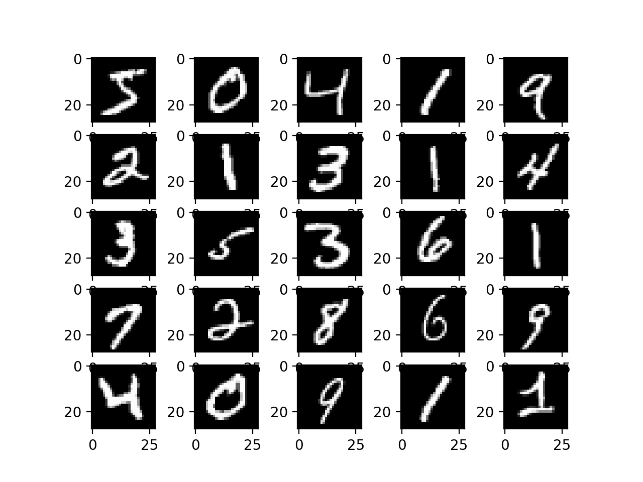
A popular image classification task is the MNIST handwritten digit classification. It involves tens of thousands of handwritten digits that must be classified as a number between 0 and 9.

The tf.keras API provides a convenience function to download and load this dataset directly.

The example below loads the dataset and plots the first few images.

# example of loading and plotting the mnist dataset
from tensorflow.keras.datasets.mnist import load_data
from matplotlib import pyplot
# load dataset
(trainX, trainy), (testX, testy) = load_data()
# summarize loaded dataset
print('Train: X=%s, y=%s' % (trainX.shape, trainy.shape))
print('Test: X=%s, y=%s' % (testX.shape, testy.shape))
# plot first few images
for i in range(25):
	# define subplot
	pyplot.subplot(5, 5, i+1)
	# plot raw pixel data
	pyplot.imshow(trainX[i], cmap=pyplot.get_cmap('gray'))
# show the figure
pyplot.show()

Running the example loads the MNIST dataset, then summarizes the default train and test datasets.

Train: X=(60000, 28, 28), y=(60000,)
Test: X=(10000, 28, 28), y=(10000,)

A plot is then created showing a grid of examples of handwritten images in the training dataset.

Plot of Handwritten Digits From the MNIST dataset

We can train a CNN model to classify the images in the MNIST dataset.

Note that the images are arrays of grayscale pixel data; therefore, we must add a channel dimension to the data before we can use the images as input to the model. The reason is that CNN models expect images in a channels-last format, that is each example to the network has the dimensions [rows, columns, channels], where channels represent the color channels of the image data.

It is also a good idea to scale the pixel values from the default range of 0-255 to 0-1 when training a CNN. For more on scaling pixel values, see the tutorial:

• How to Manually Scale Image Pixel Data for Deep Learning

The complete example of fitting and evaluating a CNN model on the MNIST dataset is listed below.

# example of a cnn for image classification
from numpy import unique
from numpy import argmax
from tensorflow.keras.datasets.mnist import load_data
from tensorflow.keras import Sequential
from tensorflow.keras.layers import Dense
from tensorflow.keras.layers import Conv2D
from tensorflow.keras.layers import MaxPooling2D
from tensorflow.keras.layers import Flatten
from tensorflow.keras.layers import Dropout
# load dataset
(x_train, y_train), (x_test, y_test) = load_data()
# reshape data to have a single channel
x_train = x_train.reshape((x_train.shape[0], x_train.shape[1], x_train.shape[2], 1))
x_test = x_test.reshape((x_test.shape[0], x_test.shape[1], x_test.shape[2], 1))
# determine the shape of the input images
in_shape = x_train.shape[1:]
# determine the number of classes
n_classes = len(unique(y_train))
print(in_shape, n_classes)
# normalize pixel values
x_train = x_train.astype('float32') / 255.0
x_test = x_test.astype('float32') / 255.0
# define model
model = Sequential()
model.add(Conv2D(32, (3,3), activation='relu', kernel_initializer='he_uniform', input_shape=in_shape))
model.add(MaxPooling2D((2, 2)))
model.add(Flatten())
model.add(Dense(100, activation='relu', kernel_initializer='he_uniform'))
model.add(Dropout(0.5))
model.add(Dense(n_classes, activation='softmax'))
# define loss and optimizer
model.compile(optimizer='adam', loss='sparse_categorical_crossentropy', metrics=['accuracy'])
# fit the model
model.fit(x_train, y_train, epochs=10, batch_size=128, verbose=0)
# evaluate the model
loss, acc = model.evaluate(x_test, y_test, verbose=0)
print('Accuracy: %.3f' % acc)
# make a prediction
image = x_train[0]
yhat = model.predict([[image]])
print('Predicted: class=%d' % argmax(yhat))

Running the example first reports the shape of the dataset, then fits the model and evaluates it on the test dataset. Finally, a prediction is made for a single image.

Your specific results will vary given the stochastic nature of the learning algorithm. Try running the example a few times.

What results did you get? Can you change the model to do better?
Post your findings to the comments below.

First, the shape of each image is reported along with the number of classes; we can see that each image is 28×28 pixels and there are 10 classes as we expected.

In this case, we can see that the model achieved a classification accuracy of about 98 percent on the test dataset. We can then see that the model predicted class 5 for the first image in the training set.

(28, 28, 1) 10
Accuracy: 0.987
Predicted: class=5

3.3 Develop Recurrent Neural Network Models

Recurrent Neural Networks, or RNNs for short, are designed to operate upon sequences of data.

They have proven to be very effective for natural language processing problems where sequences of text are provided as input to the model. RNNs have also seen some modest success for time series forecasting and speech recognition.

The most popular type of RNN is the Long Short-Term Memory network, or LSTM for short. LSTMs can be used in a model to accept a sequence of input data and make a prediction, such as assign a class label or predict a numerical value like the next value or values in the sequence.

We will use the car sales dataset to demonstrate an LSTM RNN for univariate time series forecasting.

This problem involves predicting the number of car sales per month.

The dataset will be downloaded automatically using Pandas, but you can learn more about it here.

• Car Sales Dataset (csv).
• Car Sales Dataset Description (csv).

We will frame the problem to take a window of the last five months of data to predict the current month’s data.

To achieve this, we will define a new function named split_sequence() that will split the input sequence into windows of data appropriate for fitting a supervised learning model, like an LSTM.

For example, if the sequence was:

1, 2, 3, 4, 5, 6, 7, 8, 9, 10

Then the samples for training the model will look like:

Input 				Output
1, 2, 3, 4, 5 		6
2, 3, 4, 5, 6 		7
3, 4, 5, 6, 7 		8
...

We will use the last 12 months of data as the test dataset.

LSTMs expect each sample in the dataset to have two dimensions; the first is the number of time steps (in this case it is 5), and the second is the number of observations per time step (in this case it is 1).

Because it is a regression type problem, we will use a linear activation function (no activation
function) in the output layer and optimize the mean squared error loss function. We will also evaluate the model using the mean absolute error (MAE) metric.

The complete example of fitting and evaluating an LSTM for a univariate time series forecasting problem is listed below.

# lstm for time series forecasting
from numpy import sqrt
from numpy import asarray
from pandas import read_csv
from tensorflow.keras import Sequential
from tensorflow.keras.layers import Dense
from tensorflow.keras.layers import LSTM

# split a univariate sequence into samples
def split_sequence(sequence, n_steps):
	X, y = list(), list()
	for i in range(len(sequence)):
		# find the end of this pattern
		end_ix = i + n_steps
		# check if we are beyond the sequence
		if end_ix > len(sequence)-1:
			break
		# gather input and output parts of the pattern
		seq_x, seq_y = sequence[i:end_ix], sequence[end_ix]
		X.append(seq_x)
		y.append(seq_y)
	return asarray(X), asarray(y)

# load the dataset
path = 'https://raw.githubusercontent.com/jbrownlee/Datasets/master/monthly-car-sales.csv'
df = read_csv(path, header=0, index_col=0, squeeze=True)
# retrieve the values
values = df.values.astype('float32')
# specify the window size
n_steps = 5
# split into samples
X, y = split_sequence(values, n_steps)
# reshape into [samples, timesteps, features]
X = X.reshape((X.shape[0], X.shape[1], 1))
# split into train/test
n_test = 12
X_train, X_test, y_train, y_test = X[:-n_test], X[-n_test:], y[:-n_test], y[-n_test:]
print(X_train.shape, X_test.shape, y_train.shape, y_test.shape)
# define model
model = Sequential()
model.add(LSTM(100, activation='relu', kernel_initializer='he_normal', input_shape=(n_steps,1)))
model.add(Dense(50, activation='relu', kernel_initializer='he_normal'))
model.add(Dense(50, activation='relu', kernel_initializer='he_normal'))
model.add(Dense(1))
# compile the model
model.compile(optimizer='adam', loss='mse', metrics=['mae'])
# fit the model
model.fit(X_train, y_train, epochs=350, batch_size=32, verbose=2, validation_data=(X_test, y_test))
# evaluate the model
mse, mae = model.evaluate(X_test, y_test, verbose=0)
print('MSE: %.3f, RMSE: %.3f, MAE: %.3f' % (mse, sqrt(mse), mae))
# make a prediction
row = asarray([18024.0, 16722.0, 14385.0, 21342.0, 17180.0]).reshape((1, n_steps, 1))
yhat = model.predict(row)
print('Predicted: %.3f' % (yhat))

Running the example first reports the shape of the dataset, then fits the model and evaluates it on the test dataset. Finally, a prediction is made for a single example.

Your specific results will vary given the stochastic nature of the learning algorithm. Try running the example a few times.

What results did you get? Can you change the model to do better?
Post your findings to the comments below.

First, the shape of the train and test datasets is displayed, confirming that the last 12 examples are used for model evaluation.

In this case, the model achieved an MAE of about 2,800 and predicted the next value in the sequence from the test set as 13,199, where the expected value is 14,577 (pretty close).

(91, 5, 1) (12, 5, 1) (91,) (12,)
MSE: 12755421.000, RMSE: 3571.473, MAE: 2856.084
Predicted: 13199.325

Note: it is good practice to scale and make the series stationary the data prior to fitting the model. I recommend this as an extension in order to achieve better performance. For more on preparing time series data for modeling, see the tutorial:

• 4 Common Machine Learning Data Transforms for Time Series Forecasting

4. How to Use Advanced Model Features

In this section, you will discover how to use some of the slightly more advanced model features, such as reviewing learning curves and saving models for later use.

4.1 How to Visualize a Deep Learning Model

The architecture of deep learning models can quickly become large and complex.

As such, it is important to have a clear idea of the connections and data flow in your model. This is especially important if you are using the functional API to ensure you have indeed connected the layers of the model in the way you intended.

There are two tools you can use to visualize your model: a text description and a plot.

Model Text Description

A text description of your model can be displayed by calling the summary() function on your model.

The example below defines a small model with three layers and then summarizes the structure.

# example of summarizing a model
from tensorflow.keras import Sequential
from tensorflow.keras.layers import Dense
# define model
model = Sequential()
model.add(Dense(10, activation='relu', kernel_initializer='he_normal', input_shape=(8,)))
model.add(Dense(8, activation='relu', kernel_initializer='he_normal'))
model.add(Dense(1, activation='sigmoid'))
# summarize the model
model.summary()

Running the example prints a summary of each layer, as well as a total summary.

This is an invaluable diagnostic for checking the output shapes and number of parameters (weights) in your model.

Model: "sequential"
_________________________________________________________________
Layer (type)                 Output Shape              Param #
=================================================================
dense (Dense)                (None, 10)                90
_________________________________________________________________
dense_1 (Dense)              (None, 8)                 88
_________________________________________________________________
dense_2 (Dense)              (None, 1)                 9
=================================================================
Total params: 187
Trainable params: 187
Non-trainable params: 0
_________________________________________________________________

Model Architecture Plot

You can create a plot of your model by calling the plot_model() function.

This will create an image file that contains a box and line diagram of the layers in your model.

The example below creates a small three-layer model and saves a plot of the model architecture to ‘model.png‘ that includes input and output shapes.

# example of plotting a model
from tensorflow.keras import Sequential
from tensorflow.keras.layers import Dense
from tensorflow.keras.utils import plot_model
# define model
model = Sequential()
model.add(Dense(10, activation='relu', kernel_initializer='he_normal', input_shape=(8,)))
model.add(Dense(8, activation='relu', kernel_initializer='he_normal'))
model.add(Dense(1, activation='sigmoid'))
# summarize the model
plot_model(model, 'model.png', show_shapes=True)

Running the example creates a plot of the model showing a box for each layer with shape information, and arrows that connect the layers, showing the flow of data through the network.

Plot of Neural Network Architecture

4.2 How to Plot Model Learning Curves

Learning curves are a plot of neural network model performance over time, such as calculated at the end of each training epoch.

Plots of learning curves provide insight into the learning dynamics of the model, such as whether the model is learning well, whether it is underfitting the training dataset, or whether it is overfitting the training dataset.

For a gentle introduction to learning curves and how to use them to diagnose learning dynamics of models, see the tutorial:

• How to use Learning Curves to Diagnose Machine Learning Model Performance

You can easily create learning curves for your deep learning models.

First, you must update your call to the fit function to include reference to a validation dataset. This is a portion of the training set not used to fit the model, and is instead used to evaluate the performance of the model during training.

You can split the data manually and specify the validation_data argument, or you can use the validation_split argument and specify a percentage split of the training dataset and let the API perform the split for you. The latter is simpler for now.

The fit function will return a history object that contains a trace of performance metrics recorded at the end of each training epoch. This includes the chosen loss function and each configured metric, such as accuracy, and each loss and metric is calculated for the training and validation datasets.

A learning curve is a plot of the loss on the training dataset and the validation dataset. We can create this plot from the history object using the Matplotlib library.

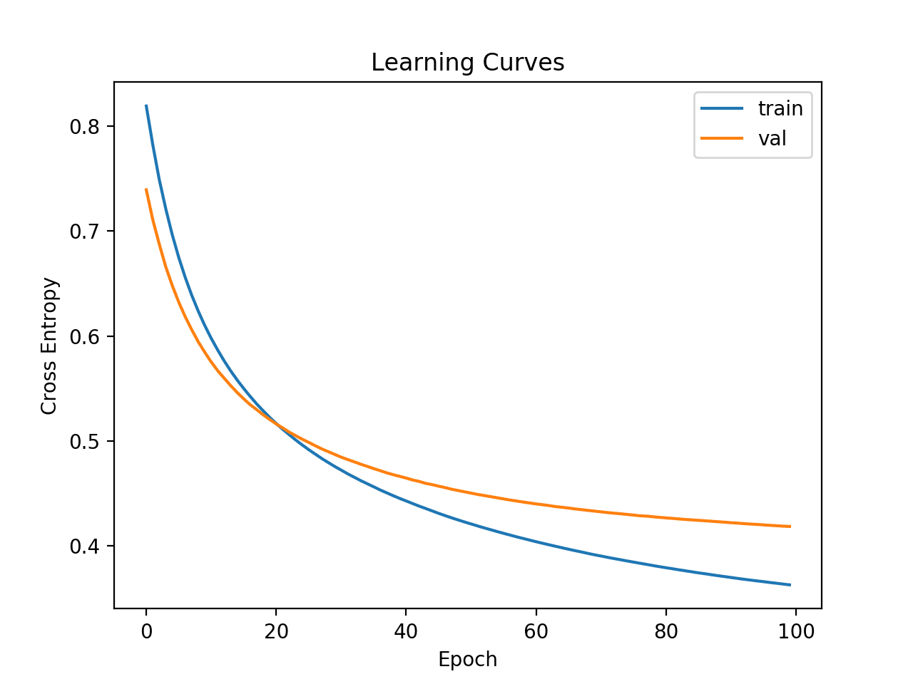
The example below fits a small neural network on a synthetic binary classification problem. A validation split of 30 percent is used to evaluate the model during training and the cross-entropy loss on the train and validation datasets are then graphed using a line plot.

# example of plotting learning curves
from sklearn.datasets import make_classification
from tensorflow.keras import Sequential
from tensorflow.keras.layers import Dense
from tensorflow.keras.optimizers import SGD
from matplotlib import pyplot
# create the dataset
X, y = make_classification(n_samples=1000, n_classes=2, random_state=1)
# determine the number of input features
n_features = X.shape[1]
# define model
model = Sequential()
model.add(Dense(10, activation='relu', kernel_initializer='he_normal', input_shape=(n_features,)))
model.add(Dense(1, activation='sigmoid'))
# compile the model
sgd = SGD(learning_rate=0.001, momentum=0.8)
model.compile(optimizer=sgd, loss='binary_crossentropy')
# fit the model
history = model.fit(X, y, epochs=100, batch_size=32, verbose=0, validation_split=0.3)
# plot learning curves
pyplot.title('Learning Curves')
pyplot.xlabel('Epoch')
pyplot.ylabel('Cross Entropy')
pyplot.plot(history.history['loss'], label='train')
pyplot.plot(history.history['val_loss'], label='val')
pyplot.legend()
pyplot.show()

Running the example fits the model on the dataset. At the end of the run, the history object is returned and used as the basis for creating the line plot.

The cross-entropy loss for the training dataset is accessed via the ‘loss‘ key and the loss on the validation dataset is accessed via the ‘val_loss‘ key on the history attribute of the history object.

Learning Curves of Cross-Entropy Loss for a Deep Learning Model

4.3 How to Save and Load Your Model

Training and evaluating models is great, but we may want to use a model later without retraining it each time.

This can be achieved by saving the model to file and later loading it and using it to make predictions.

This can be achieved using the save() function on the model to save the model. It can be loaded later using the load_model() function.

The model is saved in H5 format, an efficient array storage format. As such, you must ensure that the h5py library is installed on your workstation. This can be achieved using pip; for example:

pip install h5py

The example below fits a simple model on a synthetic binary classification problem and then saves the model file.

# example of saving a fit model
from sklearn.datasets import make_classification
from tensorflow.keras import Sequential
from tensorflow.keras.layers import Dense
from tensorflow.keras.optimizers import SGD
# create the dataset
X, y = make_classification(n_samples=1000, n_features=4, n_classes=2, random_state=1)
# determine the number of input features
n_features = X.shape[1]
# define model
model = Sequential()
model.add(Dense(10, activation='relu', kernel_initializer='he_normal', input_shape=(n_features,)))
model.add(Dense(1, activation='sigmoid'))
# compile the model
sgd = SGD(learning_rate=0.001, momentum=0.8)
model.compile(optimizer=sgd, loss='binary_crossentropy')
# fit the model
model.fit(X, y, epochs=100, batch_size=32, verbose=0, validation_split=0.3)
# save model to file
model.save('model.h5')

Running the example fits the model and saves it to file with the name ‘model.h5‘.

We can then load the model and use it to make a prediction, or continue training it, or do whatever we wish with it.

The example below loads the model and uses it to make a prediction.

# example of loading a saved model
from sklearn.datasets import make_classification
from tensorflow.keras.models import load_model
# create the dataset
X, y = make_classification(n_samples=1000, n_features=4, n_classes=2, random_state=1)
# load the model from file
model = load_model('model.h5')
# make a prediction
row = [1.91518414, 1.14995454, -1.52847073, 0.79430654]
yhat = model.predict([row])
print('Predicted: %.3f' % yhat[0])

Running the example loads the image from file, then uses it to make a prediction on a new row of data and prints the result.

Predicted: 0.831

5. How to Get Better Model Performance

In this section, you will discover some of the techniques that you can use to improve the performance of your deep learning models.

A big part of improving deep learning performance involves avoiding overfitting by slowing down the learning process or stopping the learning process at the right time.

5.1 How to Reduce Overfitting With Dropout

Dropout is a clever regularization method that reduces overfitting of the training dataset and makes the model more robust.

This is achieved during training, where some number of layer outputs are randomly ignored or “dropped out.” This has the effect of making the layer look like – and be treated like – a layer with a different number of nodes and connectivity to the prior layer.

Dropout has the effect of making the training process noisy, forcing nodes within a layer to probabilistically take on more or less responsibility for the inputs.

For more on how dropout works, see this tutorial:

• A Gentle Introduction to Dropout for Regularizing Deep Neural Networks

You can add dropout to your models as a new layer prior to the layer that you want to have input connections dropped-out.

This involves adding a layer called Dropout() that takes an argument that specifies the probability that each output from the previous to drop. E.g. 0.4 means 40 percent of inputs will be dropped each update to the model.

You can add Dropout layers in MLP, CNN, and RNN models, although there are also specialized versions of dropout for use with CNN and RNN models that you might also want to explore.

The example below fits a small neural network model on a synthetic binary classification problem.

A dropout layer with 50 percent dropout is inserted between the first hidden layer and the output layer.

# example of using dropout
from sklearn.datasets import make_classification
from tensorflow.keras import Sequential
from tensorflow.keras.layers import Dense
from tensorflow.keras.layers import Dropout
from matplotlib import pyplot
# create the dataset
X, y = make_classification(n_samples=1000, n_classes=2, random_state=1)
# determine the number of input features
n_features = X.shape[1]
# define model
model = Sequential()
model.add(Dense(10, activation='relu', kernel_initializer='he_normal', input_shape=(n_features,)))
model.add(Dropout(0.5))
model.add(Dense(1, activation='sigmoid'))
# compile the model
model.compile(optimizer='adam', loss='binary_crossentropy')
# fit the model
model.fit(X, y, epochs=100, batch_size=32, verbose=0)

5.2 How to Accelerate Training With Batch Normalization

The scale and distribution of inputs to a layer can greatly impact how easy or quickly that layer can be trained.

This is generally why it is a good idea to scale input data prior to modeling it with a neural network model.

Batch normalization is a technique for training very deep neural networks that standardizes the inputs to a layer for each mini-batch. This has the effect of stabilizing the learning process and dramatically reducing the number of training epochs required to train deep networks.

For more on how batch normalization works, see this tutorial:

• A Gentle Introduction to Batch Normalization for Deep Neural Networks

You can use batch normalization in your network by adding a batch normalization layer prior to the layer that you wish to have standardized inputs. You can use batch normalization with MLP, CNN, and RNN models.

This can be achieved by adding the BatchNormalization layer directly.

The example below defines a small MLP network for a binary classification prediction problem with a batch normalization layer between the first hidden layer and the output layer.

# example of using batch normalization
from sklearn.datasets import make_classification
from tensorflow.keras import Sequential
from tensorflow.keras.layers import Dense
from tensorflow.keras.layers import BatchNormalization
from matplotlib import pyplot
# create the dataset
X, y = make_classification(n_samples=1000, n_classes=2, random_state=1)
# determine the number of input features
n_features = X.shape[1]
# define model
model = Sequential()
model.add(Dense(10, activation='relu', kernel_initializer='he_normal', input_shape=(n_features,)))
model.add(BatchNormalization())
model.add(Dense(1, activation='sigmoid'))
# compile the model
model.compile(optimizer='adam', loss='binary_crossentropy')
# fit the model
model.fit(X, y, epochs=100, batch_size=32, verbose=0)

Also, tf.keras has a range of other normalization layers you might like to explore; see:

• tf.keras Normalization Layers Guide.

5.3 How to Halt Training at the Right Time With Early Stopping

Neural networks are challenging to train.

Too little training and the model is underfit; too much training and the model overfits the training dataset. Both cases result in a model that is less effective than it could be.

One approach to solving this problem is to use early stopping. This involves monitoring the loss on the training dataset and a validation dataset (a subset of the training set not used to fit the model). As soon as loss for the validation set starts to show signs of overfitting, the training process can be stopped.

For more on early stopping, see the tutorial:

• A Gentle Introduction to Early Stopping to Avoid Overtraining Neural Networks

Early stopping can be used with your model by first ensuring that you have a validation dataset. You can define the validation dataset manually via the validation_data argument to the fit() function, or you can use the validation_split and specify the amount of the training dataset to hold back for validation.

You can then define an EarlyStopping and instruct it on which performance measure to monitor, such as ‘val_loss‘ for loss on the validation dataset, and the number of epochs to observed overfitting before taking action, e.g. 5.

This configured EarlyStopping callback can then be provided to the fit() function via the “callbacks” argument that takes a list of callbacks.

This allows you to set the number of epochs to a large number and be confident that training will end as soon as the model starts overfitting. You might also like to create a learning curve to discover more insights into the learning dynamics of the run and when training was halted.

The example below demonstrates a small neural network on a synthetic binary classification problem that uses early stopping to halt training as soon as the model starts overfitting (after about 50 epochs).

# example of using early stopping
from sklearn.datasets import make_classification
from tensorflow.keras import Sequential
from tensorflow.keras.layers import Dense
from keras.callbacks import EarlyStopping
# create the dataset
X, y = make_classification(n_samples=1000, n_classes=2, random_state=1)
# determine the number of input features
n_features = X.shape[1]
# define model
model = Sequential()
model.add(Dense(10, activation='relu', kernel_initializer='he_normal', input_shape=(n_features,)))
model.add(Dense(1, activation='sigmoid'))
# compile the model
model.compile(optimizer='adam', loss='binary_crossentropy')
# configure early stopping
es = EarlyStopping(monitor='val_loss', patience=5)
# fit the model
history = model.fit(X, y, epochs=200, batch_size=32, verbose=0, validation_split=0.3, callbacks=[es])

The tf.keras API provides a number of callbacks that you might like to explore; you can learn more here:

• tf.keras Callbacks

Further Reading

This section provides more resources on the topic if you are looking to go deeper.

Tutorials

• How to Control the Stability of Training Neural Networks With the Batch Size
• A Gentle Introduction to the Rectified Linear Unit (ReLU)
• Difference Between Classification and Regression in Machine Learning
• How to Manually Scale Image Pixel Data for Deep Learning
• 4 Common Machine Learning Data Transforms for Time Series Forecasting
• How to use Learning Curves to Diagnose Machine Learning Model Performance
• A Gentle Introduction to Dropout for Regularizing Deep Neural Networks
• A Gentle Introduction to Batch Normalization for Deep Neural Networks
• A Gentle Introduction to Early Stopping to Avoid Overtraining Neural Networks

Books

• Deep Learning, 2016.

Guides

• Install TensorFlow 2 Guide.
• TensorFlow Core: Keras
• Tensorflow Core: Keras Overview Guide
• The Keras functional API in TensorFlow
• Save and load models
• Normalization Layers Guide.

APIs

• tf.keras Module API.
• tf.keras Optimizers
• tf.keras Loss Functions
• tf.keras Metrics

Summary

In this tutorial, you discovered a step-by-step guide to developing deep learning models in TensorFlow using the tf.keras API.

Specifically, you learned:

• The difference between Keras and tf.keras and how to install and confirm TensorFlow is working.
• The 5-step life-cycle of tf.keras models and how to use the sequential and functional APIs.
• How to develop MLP, CNN, and RNN models with tf.keras for regression, classification, and time series forecasting.
• How to use the advanced features of the tf.keras API to inspect and diagnose your model.
• How to improve the performance of your tf.keras model by reducing overfitting and accelerating training.

Do you have any questions?
Ask your questions in the comments below and I will do my best to answer.

The post TensorFlow 2 Tutorial: Get Started in Deep Learning With tf.keras appeared first on Machine Learning Mastery.

You must prepare your raw data using data transforms prior to fitting a machine learning model.

This is required to ensure that you best expose the structure of your predictive modeling problem to the learning algorithms.

Applying data transforms like scaling or encoding categorical variables is straightforward when all input variables are the same type. It can be challenging when you have a dataset with mixed types and you want to selectively apply data transforms to some, but not all, input features.

Thankfully, the scikit-learn Python machine learning library provides the ColumnTransformer that allows you to selectively apply data transforms to different columns in your dataset.

In this tutorial, you will discover how to use the ColumnTransformer to selectively apply data transforms to columns in a dataset with mixed data types.

After completing this tutorial, you will know:

• The challenge of using data transformations with datasets that have mixed data types.
• How to define, fit, and use the ColumnTransformer to selectively apply data transforms to columns.
• How to work through a real dataset with mixed data types and use the ColumnTransformer to apply different transforms to categorical and numerical data columns.

Let’s get started.

Use the ColumnTransformer for Numerical and Categorical Data in Python
Photo by Kari, some rights reserved.

Tutorial Overview

This tutorial is divided into three parts; they are:

1. Challenge of Transforming Different Data Types
2. How to use the ColumnTransformer
3. Data Preparation for the Abalone Regression Dataset

Challenge of Transforming Different Data Types

It is important to prepare data prior to modeling.

This may involve replacing missing values, scaling numerical values, and one hot encoding categorical data.

Data transforms can be performed using the scikit-learn library; for example, the SimpleImputer class can be used to replace missing values, the MinMaxScaler class can be used to scale numerical values, and the OneHotEncoder can be used to encode categorical variables.

For example:

...
# prepare transform
scaler = MinMaxScaler()
# fit transform on training data
scaler.fit(train_X)
# transform training data
train_X = scaler.transform(train_X)

Sequences of different transforms can also be chained together using the Pipeline, such as imputing missing values, then scaling numerical values.

For example:

...
# define pipeline
pipeline = Pipeline(steps=[('i', SimpleImputer(strategy='median')), ('s', MinMaxScaler())])
# transform training data
train_X = scaler.fit_transform(train_X)

It is very common to want to perform different data preparation techniques on different columns in your input data.

For example, you may want to impute missing numerical values with a median value, then scale the values and impute missing categorical values using the most frequent value and one hot encode the categories.

Traditionally, this would require you to separate the numerical and categorical data and then manually apply the transforms on those groups of features before combining the columns back together in order to fit and evaluate a model.

Now, you can use the ColumnTransformer to perform this operation for you.

How to use the ColumnTransformer

The ColumnTransformer is a class in the scikit-learn Python machine learning library that allows you to selectively apply data preparation transforms.

For example, it allows you to apply a specific transform or sequence of transforms to just the numerical columns, and a separate sequence of transforms to just the categorical columns.

To use the ColumnTransformer, you must specify a list of transformers.

Each transformer is a three-element tuple that defines the name of the transformer, the transform to apply, and the column indices to apply it to. For example:

• (Name, Object, Columns)

For example, the ColumnTransformer below applies a OneHotEncoder to columns 0 and 1.

transformer = ColumnTransformer(transformers=[('cat', OneHotEncoder(), [0, 1])])

The example below applies a SimpleImputer with median imputing for numerical columns 0 and 1, and SimpleImputer with most frequent imputing to categorical columns 2 and 3.

t = [('num', SimpleImputer(strategy='median'), [0, 1]), ('cat', SimpleImputer(strategy='most_frequent'), [2, 3])]
transformer = ColumnTransformer(transformers=t)

Any columns not specified in the list of “transformers” are dropped from the dataset by default; this can be changed by setting the “remainder” argument.

Setting remainder=’passthrough’ will mean that all columns not specified in the list of “transformers” will be passed through without transformation, instead of being dropped.

For example, if columns 0 and 1 were numerical and columns 2 and 3 were categorical and we wanted to just transform the categorical data and pass through the numerical columns unchanged, we could define the ColumnTransformer as follows:

transformer = ColumnTransformer(transformers=[('cat', OneHotEncoder(), [2, 3])], remainder='passthrough')

Once the transformer is defined, it can be used to transform a dataset.

For example:

...
transformer = ColumnTransformer(transformers=[('cat', OneHotEncoder(), [0, 1])])
# transform training data
train_X = transformer.fit_transform(train_X)

A ColumnTransformer can also be used in a Pipeline to selectively prepare the columns of your dataset before fitting a model on the transformed data.

This is the most likely use case as it ensures that the transforms are performed automatically on the raw data when fitting the model and when making predictions, such as when evaluating the model on a test dataset via cross-validation or making predictions on new data in the future.

For example:

...
# define model
model = LogisticRegression()
# define transform
transformer = ColumnTransformer(transformers=[('cat', OneHotEncoder(), [0, 1])])
# define pipeline
pipeline = Pipeline(steps=[('t', transformer), ('m',model)])
# fit the model on the transformed data
model.fit(train_X, train_y)
# make predictions
yhat = model.predict(test_X)

Now that we are familiar with how to configure and use the ColumnTransformer in general, let’s look at a worked example.

Data Preparation for the Abalone Regression Dataset

The abalone dataset is a standard machine learning problem that involves predicting the age of an abalone given measurements of an abalone.

You can download the dataset and learn more about it here:

• Download Abalone Dataset (abalone.csv)
• Learn More About the Abalone Dataset (abalone.names)

The dataset has 4,177 examples, 8 input variables, and the target variable is an integer.

A naive model can achieve a mean absolute error (MAE) of about 2.363 (std 0.092) by predicting the mean value, evaluated via 10-fold cross-validation.

We can model this as a regression predictive modeling problem with a support vector machine model (SVR).

Reviewing the data, you can see the first few rows as follows:

M,0.455,0.365,0.095,0.514,0.2245,0.101,0.15,15
M,0.35,0.265,0.09,0.2255,0.0995,0.0485,0.07,7
F,0.53,0.42,0.135,0.677,0.2565,0.1415,0.21,9
M,0.44,0.365,0.125,0.516,0.2155,0.114,0.155,10
I,0.33,0.255,0.08,0.205,0.0895,0.0395,0.055,7
...

We can see that the first column is categorical and the remainder of the columns are numerical.

We may want to one hot encode the first column and normalize the remaining numerical columns, and this can be achieved using the ColumnTransformer.

First, we need to load the dataset. We can load the dataset directly from the URL using the read_csv() Pandas function, then split the data into two data frames: one for input and one for the output.

The complete example of loading the dataset is listed below.

# load the dataset
from pandas import read_csv
# load dataset
url = 'https://raw.githubusercontent.com/jbrownlee/Datasets/master/abalone.csv'
dataframe = read_csv(url, header=None)
# split into inputs and outputs
last_ix = len(dataframe.columns) - 1
X, y = dataframe.drop(last_ix, axis=1), dataframe[last_ix]
print(X.shape, y.shape)

Note: if you have trouble loading the dataset from a URL, you can download the CSV file with the name ‘abalone.csv‘ and place it in the same directory as your Python file and change the call to read_csv() as follows:

...
dataframe = read_csv('abalone.csv', header=None)

Running the example, we can see that the dataset is loaded correctly and split into eight input columns and one target column.

(4177, 8) (4177,)

Next, we can use the select_dtypes() function to select the column indexes that match different data types.

We are interested in a list of columns that are numerical columns marked as ‘float64‘ or ‘int64‘ in Pandas, and a list of categorical columns, marked as ‘object‘ or ‘bool‘ type in Pandas.

...
# determine categorical and numerical features
numerical_ix = X.select_dtypes(include=['int64', 'float64']).columns
categorical_ix = X.select_dtypes(include=['object', 'bool']).columns

We can then use these lists in the ColumnTransformer to one hot encode the categorical variables, which should just be the first column.

We can also use the list of numerical columns to normalize the remaining data.

...
# define the data preparation for the columns
t = [('cat', OneHotEncoder(), categorical_ix), ('num', MinMaxScaler(), numerical_ix)]
col_transform = ColumnTransformer(transformers=t)

Next, we can define our SVR model and define a Pipeline that first uses the ColumnTransformer, then fits the model on the prepared dataset.

...
# define the model
model = SVR(kernel='rbf',gamma='scale',C=100)
# define the data preparation and modeling pipeline
pipeline = Pipeline(steps=[('prep',col_transform), ('m', model)])

Finally, we can evaluate the model using 10-fold cross-validation and calculate the mean absolute error, averaged across all 10 evaluations of the pipeline.

...
# define the model cross-validation configuration
cv = KFold(n_splits=10, shuffle=True, random_state=1)
# evaluate the pipeline using cross validation and calculate MAE
scores = cross_val_score(pipeline, X, y, scoring='neg_mean_absolute_error', cv=cv, n_jobs=-1)
# convert MAE scores to positive values
scores = absolute(scores)
# summarize the model performance
print('MAE: %.3f (%.3f)' % (mean(scores), std(scores)))

Tying this all together, the complete example is listed below.

# example of using the ColumnTransformer for the Abalone dataset
from numpy import mean
from numpy import std
from numpy import absolute
from pandas import read_csv
from sklearn.model_selection import cross_val_score
from sklearn.model_selection import KFold
from sklearn.compose import ColumnTransformer
from sklearn.pipeline import Pipeline
from sklearn.preprocessing import OneHotEncoder
from sklearn.preprocessing import MinMaxScaler
from sklearn.svm import SVR

# load dataset
url = 'https://raw.githubusercontent.com/jbrownlee/Datasets/master/abalone.csv'
dataframe = read_csv(url, header=None)
# split into inputs and outputs
last_ix = len(dataframe.columns) - 1
X, y = dataframe.drop(last_ix, axis=1), dataframe[last_ix]
print(X.shape, y.shape)
# determine categorical and numerical features
numerical_ix = X.select_dtypes(include=['int64', 'float64']).columns
categorical_ix = X.select_dtypes(include=['object', 'bool']).columns
# define the data preparation for the columns
t = [('cat', OneHotEncoder(), categorical_ix), ('num', MinMaxScaler(), numerical_ix)]
col_transform = ColumnTransformer(transformers=t)
# define the model
model = SVR(kernel='rbf',gamma='scale',C=100)
# define the data preparation and modeling pipeline
pipeline = Pipeline(steps=[('prep',col_transform), ('m', model)])
# define the model cross-validation configuration
cv = KFold(n_splits=10, shuffle=True, random_state=1)
# evaluate the pipeline using cross validation and calculate MAE
scores = cross_val_score(pipeline, X, y, scoring='neg_mean_absolute_error', cv=cv, n_jobs=-1)
# convert MAE scores to positive values
scores = absolute(scores)
# summarize the model performance
print('MAE: %.3f (%.3f)' % (mean(scores), std(scores)))

Running the example evaluates the data preparation pipeline using 10-fold cross-validation.

Your specific results may vary given the stochastic learning algorithm and differences in library versions.

In this case, we achieve an average MAE of about 1.4, which is better than the baseline score of 2.3.

(4177, 8) (4177,)
MAE: 1.465 (0.047)

You now have a template for using the ColumnTransformer on a dataset with mixed data types that you can use and adapt for your own projects in the future.

Further Reading

This section provides more resources on the topic if you are looking to go deeper.

API

• sklearn.compose.ColumnTransformer API.
• pandas.read_csv API.
• sklearn.impute.SimpleImputer API.
• sklearn.preprocessing.OneHotEncoder API.
• sklearn.preprocessing.MinMaxScaler API
• sklearn.pipeline.Pipeline API.

Summary

In this tutorial, you discovered how to use the ColumnTransformer to selectively apply data transforms to columns in datasets with mixed data types.

Specifically, you learned:

• The challenge of using data transformations with datasets that have mixed data types.
• How to define, fit, and use the ColumnTransformer to selectively apply data transforms to columns.
• How to work through a real dataset with mixed data types and use the ColumnTransformer to apply different transforms to categorical and numerical data columns.

Do you have any questions?
Ask your questions in the comments below and I will do my best to answer.

The post Use the ColumnTransformer for Numerical and Categorical Data in Python appeared first on Machine Learning Mastery.

Classification predictive modeling involves predicting a class label for a given observation.

An imbalanced classification problem is an example of a classification problem where the distribution of examples across the known classes is biased or skewed. The distribution can vary from a slight bias to a severe imbalance where there is one example in the minority class for hundreds, thousands, or millions of examples in the majority class or classes.

Imbalanced classifications pose a challenge for predictive modeling as most of the machine learning algorithms used for classification were designed around the assumption of an equal number of examples for each class. This results in models that have poor predictive performance, specifically for the minority class. This is a problem because typically, the minority class is more important and therefore the problem is more sensitive to classification errors for the minority class than the majority class.

In this tutorial, you will discover imbalanced classification predictive modeling.

After completing this tutorial, you will know:

• Imbalanced classification is the problem of classification when there is an unequal distribution of classes in the training dataset.
• The imbalance in the class distribution may vary, but a severe imbalance is more challenging to model and may require specialized techniques.
• Many real-world classification problems have an imbalanced class distribution, such as fraud detection, spam detection, and churn prediction.

Let’s get started.

A Gentle Introduction to Imbalanced Classification
Photo by John Mason, some rights reserved.

Tutorial Overview

This tutorial is divided into five parts; they are:

1. Classification Predictive Modeling
2. Imbalanced Classification Problems
3. Causes of Class Imbalance
4. Challenge of Imbalanced Classification
5. Examples of Imbalanced Classification

Classification Predictive Modeling

Classification is a predictive modeling problem that involves assigning a class label to each observation.

… classification models generate a predicted class, which comes in the form of a discrete category. For most practical applications, a discrete category prediction is required in order to make a decision.

— Page 248, Applied Predictive Modeling, 2013.

Each example is comprised of both the observations and a class label.

• Example: An observation from the domain (input) and an associated class label (output).

For example, we may collect measurements of a flower and classify the species of flower (label) from the measurements. The number of classes for a predictive modeling problem is typically fixed when the problem is framed or described, and typically, the number of classes does not change.

We may alternately choose to predict a probability of class membership instead of a crisp class label.

This allows a predictive model to share uncertainty in a prediction across a range of options and allow the user to interpret the result in the context of the problem.

Like regression models, classification models produce a continuous valued prediction, which is usually in the form of a probability (i.e., the predicted values of class membership for any individual sample are between 0 and 1 and sum to 1).

— Page 248, Applied Predictive Modeling, 2013.

For example, given measurements of a flower (observation), we may predict the likelihood (probability) of the flower being an example of each of twenty different species of flower.

The number of classes for a predictive modeling problem is typically fixed when the problem is framed or described, and usually, the number of classes does not change.

A classification predictive modeling problem may have two class labels. This is the simplest type of classification problem and is referred to as two-class classification or binary classification. Alternately, the problem may have more than two classes, such as three, 10, or even hundreds of classes. These types of problems are referred to as multi-class classification problems.

• Binary Classification Problem: A classification predictive modeling problem where all examples belong to one of two classes.
• Multiclass Classification Problem: A classification predictive modeling problem where all examples belong to one of three classes.

When working on classification predictive modeling problems, we must collect a training dataset.

A training dataset is a number of examples from the domain that include both the input data (e.g. measurements) and the output data (e.g. class label).

• Training Dataset: A number of examples collected from the problem domain that include the input observations and output class labels.

Depending on the complexity of the problem and the types of models we may choose to use, we may need tens, hundreds, thousands, or even millions of examples from the domain to constitute a training dataset.

The training dataset is used to better understand the input data to help best prepare it for modeling. It is also used to evaluate a suite of different modeling algorithms. It is used to tune the hyperparameters of a chosen model. And finally, the training dataset is used to train a final model on all available data that we can use in the future to make predictions for new examples from the problem domain.

Now that we are familiar with classification predictive modeling, let’s consider an imbalance of classes in the training dataset.

Imbalanced Classification Problems

The number of examples that belong to each class may be referred to as the class distribution.

Imbalanced classification refers to a classification predictive modeling problem where the number of examples in the training dataset for each class label is not balanced.

That is, where the class distribution is not equal or close to equal, and is instead biased or skewed.

• Imbalanced Classification: A classification predictive modeling problem where the distribution of examples across the classes is not equal.

For example, we may collect measurements of flowers and have 80 examples of one flower species and 20 examples of a second flower species, and only these examples comprise our training dataset. This represents an example of an imbalanced classification problem.

An imbalance occurs when one or more classes have very low proportions in the training data as compared to the other classes.

— Page 419, Applied Predictive Modeling, 2013.

We refer to these types of problems as “imbalanced classification” instead of “unbalanced classification“. Unbalance refers to a class distribution that was balanced and is now no longer balanced, whereas imbalanced refers to a class distribution that is inherently not balanced.

There are other less general names that may be used to describe these types of classification problems, such as:

• Rare event prediction.
• Extreme event prediction.
• Severe class imbalance.

The imbalance of a problem is defined by the distribution of classes in a specific training dataset.

… class imbalance must be defined with respect to a particular dataset or distribution. Since class labels are required in order to determine the degree of class imbalance, class imbalance is typically gauged with respect to the training distribution.

— Page 16, Imbalanced Learning: Foundations, Algorithms, and Applications, 2013.

It is common to describe the imbalance of classes in a dataset in terms of a ratio.

For example, an imbalanced binary classification problem with an imbalance of 1 to 100 (1:100) means that for every one example in one class, there are 100 examples in the other class.

Another way to describe the imbalance of classes in a dataset is to summarize the class distribution as percentages of the training dataset. For example, an imbalanced multiclass classification problem may have 80 percent examples in the first class, 18 percent in the second class, and 2 percent in a third class.

Now that we are familiar with the definition of an imbalanced classification problem, let’s look at some possible reasons as to why the classes may be imbalanced.

Causes of Class Imbalance

The imbalance to the class distribution in an imbalanced classification predictive modeling problem may have many causes.

There are perhaps two main groups of causes for the imbalance we may want to consider; they are data sampling and properties of the domain.

It is possible that the imbalance in the examples across the classes was caused by the way the examples were collected or sampled from the problem domain. This might involve biases introduced during data collection, and errors made during data collection.

• Biased Sampling.
• Measurement Errors.

For example, perhaps examples were collected from a narrow geographical region, or slice of time, and the distribution of classes may be quite different or perhaps even collected in a different way.

Errors may have been made when collecting the observations. One type of error might have been applying the wrong class labels to many examples. Alternately, the processes or systems from which examples were collected may have been damaged or impaired to cause the imbalance.

Often in cases where the imbalance is caused by a sampling bias or measurement error, the imbalance can be corrected by improved sampling methods, and/or correcting the measurement error. This is because the training dataset is not a fair representation of the problem domain that is being addressed.

The imbalance might be a property of the problem domain.

For example, the natural occurrence or presence of one class may dominate other classes. This may be because the process that generates observations in one class is more expensive in time, cost, computation, or other resources. As such, it is often infeasible or intractable to simply collect more samples from the domain in order to improve the class distribution. Instead, a model is required to learn the difference between the classes.

Now that we are familiar with the possible causes of a class imbalance, let’s consider why imbalanced classification problems are challenging.

Challenge of Imbalanced Classification

The imbalance of the class distribution will vary across problems.

A classification problem may be a little skewed, such as if there is a slight imbalance. Alternately, the classification problem may have a severe imbalance where there might be hundreds or thousands of examples in one class and tens of examples in another class for a given training dataset.

• Slight Imbalance. An imbalanced classification problem where the distribution of examples is uneven by a small amount in the training dataset (e.g. 4:6).
• Severe Imbalance. An imbalanced classification problem where the distribution of examples is uneven by a large amount in the training dataset (e.g. 1:100 or more).

Most of the contemporary works in class imbalance concentrate on imbalance ratios ranging from 1:4 up to 1:100. […] In real-life applications such as fraud detection or cheminformatics we may deal with problems with imbalance ratio ranging from 1:1000 up to 1:5000.

— Learning from imbalanced data – Open challenges and future directions, 2016.

A slight imbalance is often not a concern, and the problem can often be treated like a normal classification predictive modeling problem. A severe imbalance of the classes can be challenging to model and may require the use of specialized techniques.

Any dataset with an unequal class distribution is technically imbalanced. However, a dataset is said to be imbalanced when there is a significant, or in some cases extreme, disproportion among the number of examples of each class of the problem.

— Page 19, Learning from Imbalanced Data Sets, 2018.

The class or classes with abundant examples are called the major or majority classes, whereas the class with few examples (and there is typically just one) is called the minor or minority class.

• Majority Class: The class (or classes) in an imbalanced classification predictive modeling problem that has many examples.
• Minority Class: The class in an imbalanced classification predictive modeling problem that has few examples.

When working with an imbalanced classification problem, the minority class is typically of the most interest. This means that a model’s skill in correctly predicting the class label or probability for the minority class is more important than the majority class or classes.

Developments in learning from imbalanced data have been mainly motivated by numerous real-life applications in which we face the problem of uneven data representation. In such cases the minority class is usually the more important one and hence we require methods to improve its recognition rates.

— Learning from imbalanced data – Open challenges and future directions, 2016.

The minority class is harder to predict because there are few examples of this class, by definition. This means it is more challenging for a model to learn the characteristics of examples from this class, and to differentiate examples from this class from the majority class (or classes).

The abundance of examples from the majority class (or classes) can swamp the minority class. Most machine learning algorithms for classification predictive models are designed and demonstrated on problems that assume an equal distribution of classes. This means that a naive application of a model may focus on learning the characteristics of the abundant observations only, neglecting the examples from the minority class that is, in fact, of more interest and whose predictions are more valuable.

… the learning process of most classification algorithms is often biased toward the majority class examples, so that minority ones are not well modeled into the final system.

— Page vii, Learning from Imbalanced Data Sets, 2018.

Imbalanced classification is not “solved.”

It remains an open problem generally, and practically must be identified and addressed specifically for each training dataset.

This is true even in the face of more data, so-called “big data,” large neural network models, so-called “deep learning,” and very impressive competition-winning models, so-called “xgboost.”

Despite intense works on imbalanced learning over the last two decades there are still many shortcomings in existing methods and problems yet to be properly addressed.

— Learning from imbalanced data – Open challenges and future directions, 2016.

Now that we are familiar with the challenge of imbalanced classification, let’s look at some common examples.

Examples of Imbalanced Classification

Many of the classification predictive modeling problems that we are interested in solving in practice are imbalanced.

As such, it is surprising that imbalanced classification does not get more attention than it does.

Imbalanced learning not only presents significant new challenges to the data research community but also raises many critical questions in real-world data- intensive applications, ranging from civilian applications such as financial and biomedical data analysis to security- and defense-related applications such as surveillance and military data analysis.

— Page 2, Imbalanced Learning: Foundations, Algorithms, and Applications, 2013.

Below is a list of ten examples of problem domains where the class distribution of examples is inherently imbalanced.

Many classification problems may have a severe imbalance in the class distribution; nevertheless, looking at common problem domains that are inherently imbalanced will make the ideas and challenges of class imbalance concrete.

• Fraud Detection.
• Claim Prediction
• Default Prediction.
• Churn Prediction.
• Spam Detection.
• Anomaly Detection.
• Outlier Detection.
• Intrusion Detection
• Conversion Prediction.

The list of examples sheds light on the nature of imbalanced classification predictive modeling.

Each of these problem domains represents an entire field of study, where specific problems from each domain can be framed and explored as imbalanced classification predictive modeling. This highlights the multidisciplinary nature of class imbalanced classification, and why it is so important for a machine learning practitioner to be aware of the problem and skilled in addressing it.

Imbalance can be present in any data set or application, and hence, the practitioner should be aware of the implications of modeling this type of data.

— Page 419, Applied Predictive Modeling, 2013.

Notice that most, if not all, of the examples are likely binary classification problems. Notice too that examples from the minority class are rare, extreme, abnormal, or unusual in some way.

Also notice that many of the domains are described as “detection,” highlighting the desire to discover the minority class amongst the abundant examples of the majority class.

We now have a robust overview of imbalanced classification predictive modeling.

Further Reading

This section provides more resources on the topic if you are looking to go deeper.

Tutorials

• 8 Tactics to Combat Imbalanced Classes in Your Machine Learning Dataset
• How to Develop and Evaluate Naive Classifier Strategies Using Probability

Books

• Chapter 16: Remedies for Severe Class Imbalance, Applied Predictive Modeling, 2013.
• Imbalanced Learning: Foundations, Algorithms, and Applications, 2013.
• Learning from Imbalanced Data Sets, 2018.

Papers

• Learning from imbalanced data – Open challenges and future directions, 2016.

Articles

• Anomaly detection, Wikipedia.

Summary

In this tutorial, you discovered imbalanced classification predictive modeling.

Specifically, you learned:

• Imbalanced classification is the problem of classification when there is an unequal distribution of classes in the training dataset.
• The imbalance in the class distribution may vary, but a severe imbalance is more challenging to model and may require specialized techniques.
• Many real-world classification problems have an imbalanced class distribution such as fraud detection, spam detection, and churn prediction.

Do you have any questions?
Ask your questions in the comments below and I will do my best to answer.

The post A Gentle Introduction to Imbalanced Classification appeared first on Machine Learning Mastery.

Classification is a predictive modeling problem that involves predicting a class label for a given example.

It is generally assumed that the distribution of examples in the training dataset is even across all of the classes. In practice, this is rarely the case.

Those classification predictive models where the distribution of examples across class labels is not equal (e.g. are skewed) are called “imbalanced classification.”

Typically, a slight imbalance is not a problem and standard machine learning techniques can be used. In those cases where the imbalance is severe, such as a 1:100, 1:1000, or higher ratio of the minority to the majority class, then specialized techniques are required.

The reason why specialized techniques are required for classification problems with a severe imbalance in the classes is that most machine learning models used for classification were designed and tested around the assumption that the class distribution is equal. As such, they often fail or result in misleading results.

In this tutorial, you will discover the best resources that you can use to get started with imbalanced classification.

After completing this tutorial, you will know:

• The best books on the topic of machine learning for imbalanced classification.
• The best survey papers that introduce the topic of class imbalance.
• The best Python libraries that you can use to develop solutions for your imbalanced dataset.

Let’s get started.

Best Resources for Imbalanced Classification
Photo by Radek Kucharski, some rights reserved.

Tutorial Overview

This tutorial is divided into three parts; they are:

1. Books on Imbalanced Classification
2. Survey Papers on Imbalanced Classification
3. Python Libraries for Imbalanced Classification

Books on Imbalanced Classification

Addressing imbalanced classification predictive modeling problems with machine learning is a relatively new area of study.

Nevertheless, given the pervasiveness of imbalanced classification datasets, a few books and book chapters are available on the topic.

In this section, we will take a closer look at the following books on imbalanced classification for machine learning:

• Imbalanced Learning: Foundations, Algorithms, and Applications, 2013.
• Learning from Imbalanced Data Sets, 2018.

I will also include the following book that features a dedicated chapter on the topic:

• Applied Predictive Modeling, 2013.

There are two other books I found that are related, but perhaps more tangentially, and I won’t cover them in more detail; they were:

• Statistical Methods for Imbalanced Data in Ecological and Biological Studies, 2019.
• Dealing with Imbalanced and Weakly Labelled Data in Machine Learning using Fuzzy and Rough Set Methods, 2018.

Let’s take a closer look at the books.

Imbalanced Learning: Foundations, Algorithms, and Applications

This book is a collection of papers that form chapters, edited by two academics that have written a lot on the topic: Haibo He and Yunqian Ma.

The book was published in 2013.

• Imbalanced Learning: Foundations, Algorithms, and Applications, 2013.

Imbalanced Learning – Foundations, Algorithms, and Applications

The book is designed to bring a postgraduate student or academic up to speed with the field of imbalanced learning. This is a more general field than imbalanced classification, as it includes other problem types where the training dataset may be imbalanced, such as regression and clustering.

Specifically, we define imbalanced learning as the learning process for data representation and information extraction with severe data distribution skews to develop effective decision boundaries to support the decision-making process. The learning process could involve supervised learning, unsupervised learning, semi-supervised learning, or a combination of two or all of them. The task of imbalanced learning could also be applied to regression, classification, or clustering tasks.

— Pages 1-2, Imbalanced Learning: Foundations, Algorithms, and Applications, 2013.

It provides an excellent starting point for a practitioner to get an overview of the field and the techniques.

The table of contents for this book is listed below.

• 1. Introduction
• 2. Foundations of Imbalanced Learning
• 3. Imbalanced Datasets: From Sampling to Classifiers
• 4. Ensemble Methods for Class Imbalance Learning
• 5. Class Imbalance Learning Methods for Support Vector Machines
• 6. Class Imbalance and Active Learning
• 7. Nonstationary Stream Data Learning with Imbalanced Class Distribution
• 8. Assessment Metrics for Imbalanced Learning

Learn more about the book here.

Learning from Imbalanced Data Sets

This book is also a collection of papers on the topic of machine learning for imbalanced datasets, although feels more cohesiveness than the previous book “Imbalanced Learning.”

The book was written or edited by a laundry list of academics Alberto Fernández, Salvador García, Mikel Galar, Ronaldo Prati, Bartosz Krawczyk, and Francisco Herrera and was published in 2018.

• Learning from Imbalanced Data Sets, 2018.

Learning from Imbalanced Data Sets

Similar to the previous book, this book is designed to bring postgraduate students and engineers up to speed with the field of machine learning for imbalanced datasets.

The intended audience of this book are developers and engineers aiming to apply imbalance-learning techniques to solve different kinds of real-world problems, as well as researchers and students needing a comprehensive review on techniques, methodologies, and tools for learning from imbalanced data.

— Page viii, Learning from Imbalanced Data Sets, 2018.

The book reads as being more systematic (e.g. working through a project end-to-end) and practical than the previous book, which read as more academic (pet methods or subfields). I would recommend buying both together if you had the budget.

The table of contents for this book is listed below.

• 1. Introduction to KDD and Data Science
• 2. Foundations on Imbalanced Classification
• 3. Performance Measures
• 4. Cost-Sensitive Learning
• 5. Data Level Preprocessing Methods
• 6. Algorithm-Level Approaches
• 7. Ensemble Learning
• 8. Imbalanced Classification with Multiple Classes
• 9. Dimensionality Reduction for Imbalanced Learning
• 10. Data Intrinsic Characteristics
• 11. Learning from Imbalanced Data Streams
• 12. Non-classical Imbalanced Classification Problems
• 13. Imbalanced Classification for Big Data
• 14. Software and Libraries for Imbalanced Classification

Learn more about the book here.

Applied Predictive Modeling

This is one of my favorite handbooks for applied machine learning, written by Max Kuhn and Kjell Johnson and focused on R.

The book was published in 2013, but the general advice is probably timeless.

• Applied Predictive Modeling, 2013.

Applied Predictive Modeling

Although the whole book is a great read, the book has one chapter dedicated to the problem of imbalanced classification.

• Chapter 16: Remedies for Severe Class Imbalance

The approach to the chapter is a case study on a “Caravan Policy Ownership” dataset. The authors work through this problem to demonstrate a suite of different practical techniques for handling a severe class imbalance.

This chapter is required reading for a practical demonstration on how to work through a real-world imbalanced dataset using modern methods.

The sections of this chapter are as follows:

• 16.1 Case Study: Predicting Caravan Policy Ownership
• 16.2 The Effect of Class Imbalance
• 16.3 Model Tuning
• 16.4 Alternate Cutoffs
• 16.5 Adjusting Prior Probabilities
• 16.6 Unequal Case Weights
• 16.7 Sampling Methods
• 16.8 Cost-Sensitive Training
• 16.9 Computing

Learn more about the book here.

Survey Papers on Imbalanced Classification

There are thousands of publications on machine learning methods for imbalanced classification and related problems and techniques.

Instead of enumerating the best papers in the field, in this section, we will take a look at some of the best survey papers.

A survey paper is a paper that gives a broad overview of the field and position of the techniques in the field and how they might relate to each other. They are designed to help newcomers to the field, such as postgraduate students and engineers, get up-to-speed rapidly.

As a practitioner, reading a survey paper may be more efficient than skimming books on the topic.

There are many great survey papers to choose from; my recommended favorites are as follows:

• Learning From Imbalanced Data: Open Challenges And Future Directions, Bartosz Krawczyk, 2016.
• A Survey of Predictive Modelling under Imbalanced Distributions, Paula Branco, Luis Torgo, and Rita Ribeiro, 2015.
• Classification Of Imbalanced Data: A Review, Yanmin Sun, Andrew Wong, Mohamed Kamel, 2009.
• Learning from Imbalanced Data, Haibo He and Edwardo Garcia, 2009.

I also recommend study papers, papers that demonstrate one or more standard techniques against a suite of standard machine learning datasets. In this case, the techniques are designed to address the imbalanced class distribution and the standard datasets have a skewed class distribution.

These papers quickly flush out what methods work (or are popular) and what datasets are useful as benchmarks.

Some examples of good papers of this type include:

• An Insight Into Classification With Imbalanced Data: Empirical Results And Current Trends On Using Data Intrinsic Characteristics, 2013.
• A Study Of The Behavior Of Several Methods For Balancing Machine Learning Training Data, 2004.

Python Libraries for Imbalanced Classification

Python has rapidly become the preferred programming language for applied machine learning.

Scikit-Learn Library

The go-to library for machine learning in Python is scikit-learn, which provides data preparation, machine learning algorithms, and model evaluation schemes, among other techniques.

Scikit-learn is a Python module integrating a wide range of state-of-the-art machine learning algorithms for medium-scale supervised and unsupervised problems. This package focuses on bringing machine learning to non-specialists using a general-purpose high-level language.

— Scikit-learn: Machine Learning in Python, 2011.

Although not designed around the problem of imbalanced classification, the scikit-learn library does provide some tools for handling imbalanced datasets, such as:

• Support for a range of metrics, e.g. ROC AUC and precision/recall, F1, Brier Score and more.
• Support for class weighting, e.g. Decision Trees, SVM and more.

Imbalanced-Learn Library

A project related to scikit-learn dedicated to the problem of imbalanced classification is called imbalanced-learn.

It provides techniques that can be used for imbalanced classification in conjunction with the scikit-learn library, allowing learning algorithms and model evaluation techniques to be shared between the libraries.

imbalanced-learn is an open-source python toolbox aiming at providing a wide range of methods to cope with the problem of imbalanced dataset frequently encountered in machine learning and pattern recognition.

— Imbalanced-learn: A Python Toolbox to Tackle the Curse of Imbalanced Datasets in Machine Learning, 2016.

The library focuses on providing oversampling and undersampling techniques to make the class distribution more equal in a training dataset prior to fitting a given machine learning model.

For more on imbalanced-learn, see:

• imbalanced-learn Project, GitHub.
• imbalanced-learn Documentation.
• Imbalanced-learn: A Python Toolbox to Tackle the Curse of Imbalanced Datasets in Machine Learning, 2016.

Summary

In this tutorial, you discovered the best resources that you can use to get started with imbalanced classification.

Specifically, you learned:

• The best books on the topic of machine learning for imbalanced classification.
• The best survey papers that introduce the topic of class imbalance.
• The best Python libraries that you can use to develop solutions for your imbalanced dataset.

Do you have any questions?
Ask your questions in the comments below and I will do my best to answer.

The post Best Resources for Imbalanced Classification appeared first on Machine Learning Mastery.

An imbalanced classification problem is a problem that involves predicting a class label where the distribution of class labels in the training dataset is not equal.

A challenge for beginners working with imbalanced classification problems is what a specific skewed class distribution means. For example, what is the difference and implication for a 1:10 vs. a 1:100 class ratio?

Differences in the class distribution for an imbalanced classification problem will influence the choice of data preparation and modeling algorithms. Therefore it is critical that practitioners develop an intuition for the implications for different class distributions.

In this tutorial, you will discover how to develop a practical intuition for imbalanced and highly skewed class distributions.

After completing this tutorial, you will know:

• How to create a synthetic dataset for binary classification and plot the examples by class.
• How to create synthetic classification datasets with any given class distribution.
• How different skewed class distributions actually look in practice.

Let’s get started.

Develop an Intuition for Severely Skewed Class Distributions
Photo by Boris Kasimov, some rights reserved.

Tutorial Overview

This tutorial is divided into three parts; they are:

1. Create and Plot a Binary Classification Problem
2. Create Synthetic Dataset With Class Distribution
3. Effect of Skewed Class Distributions

Create and Plot a Binary Classification Problem

The scikit-learn Python machine learning library provides functions for generating synthetic datasets.

The make_blobs() function can be used to generate a specified number examples from a test classification problem with a specified number of classes. The function returns the input and output parts of each example ready for modeling.

For example, the snippet below will generate 1,000 examples for a two-class (binary) classification problem with two input variables. The class values have the values of 0 and 1.

...
X, y = make_blobs(n_samples=1000, centers=2, n_features=2, random_state=1, cluster_std=3)

Once generated, we can then plot the dataset to get an intuition for the spatial relationship between the examples.

Because there are only two input variables, we can create a scatter plot to plot each example as a point. This can be achieved with the scatter() matplotlib function.

The color of the points can then be varied based on the class values. This can be achieved by first selecting the array indexes for the examples for a given class, then only plotting those points, then repeating the select-and-plot process for the other class. The where() NumPy function can be used to retrieve the array indexes that match a criterion, such as a class label having a given value.

For example:

...
# create scatter plot for samples from each class
for class_value in range(2):
	# get row indexes for samples with this class
	row_ix = where(y == class_value)
	# create scatter of these samples
	pyplot.scatter(X[row_ix, 0], X[row_ix, 1])

Tying this together, the complete example of creating a binary classification test dataset and plotting the examples as a scatter plot is listed below.

# generate binary classification dataset and plot
from numpy import where
from matplotlib import pyplot
from sklearn.datasets.samples_generator import make_blobs
# generate dataset
X, y = make_blobs(n_samples=1000, centers=2, n_features=2, random_state=1, cluster_std=3)
# create scatter plot for samples from each class
for class_value in range(2):
	# get row indexes for samples with this class
	row_ix = where(y == class_value)
	# create scatter of these samples
	pyplot.scatter(X[row_ix, 0], X[row_ix, 1])
# show the plot
pyplot.show()

Running the example creates the dataset and scatter plot, showing the examples for each of the two classes with different colors.

We can see that there is an equal number of examples in each class, in this case, 500, and that we can imagine drawing a line to reasonably separate the classes, much like a classification predictive model might in learning how to discriminate the examples.

Scatter Plot of Binary Classification Dataset

Now that we know how to create a synthetic binary classification dataset and plot the examples, let’s look at the example of class imbalances on the example.

Create Synthetic Dataset with Class Distribution

The make_blobs() function will always create synthetic datasets with an equal class distribution.

Nevertheless, we can use this function to create synthetic classification datasets with arbitrary class distributions with a few extra lines of code.

A class distribution can be defined as a dictionary where the key is the class value (e.g. 0 or 1) and the value is the number of randomly generated examples to include in the dataset.

For example, an equal class distribution with 5,000 examples in each class would be defined as:

...
# define the class distribution
proportions = {0:5000, 1:5000}

We can then enumerate through the different distributions and find the largest distribution, then use the make_blobs() function to create a dataset with that many examples for each of the classes.

...
# determine the number of classes
n_classes = len(proportions)
# determine the number of examples to generate for each class
largest = max([v for k,v in proportions.items()])
n_samples = largest * n_classes

This is a good starting point, but will give us more samples than are required for each class label.

We can then enumerate through the class labels and select the desired number of examples for each class to comprise the dataset that will be returned.

...
# collect the examples
X_list, y_list = list(), list()
for k,v in proportions.items():
	row_ix = where(y == k)[0]
	selected = row_ix[:v]
	X_list.append(X[selected, :])
	y_list.append(y[selected])

We can tie this together into a new function named get_dataset() that will take a class distribution and return a synthetic dataset with that class distribution.

# create a dataset with a given class distribution
def get_dataset(proportions):
	# determine the number of classes
	n_classes = len(proportions)
	# determine the number of examples to generate for each class
	largest = max([v for k,v in proportions.items()])
	n_samples = largest * n_classes
	# create dataset
	X, y = make_blobs(n_samples=n_samples, centers=n_classes, n_features=2, random_state=1, cluster_std=3)
	# collect the examples
	X_list, y_list = list(), list()
	for k,v in proportions.items():
		row_ix = where(y == k)[0]
		selected = row_ix[:v]
		X_list.append(X[selected, :])
		y_list.append(y[selected])
	return vstack(X_list), hstack(y_list)

The function can take any number of classes, although we will use it for simple binary classification problems.

Next, we can take the code from the previous section for creating a scatter plot for a created dataset and place it in a helper function. Below is the plot_dataset() function that will plot the dataset and show a legend to indicate the mapping of colors to class labels.

# scatter plot of dataset, different color for each class
def plot_dataset(X, y):
	# create scatter plot for samples from each class
	n_classes = len(unique(y))
	for class_value in range(n_classes):
		# get row indexes for samples with this class
		row_ix = where(y == class_value)[0]
		# create scatter of these samples
		pyplot.scatter(X[row_ix, 0], X[row_ix, 1], label=str(class_value))
	# show a legend
	pyplot.legend()
	# show the plot
	pyplot.show()

Finally, we can test these new functions.

We will define a dataset with 5,000 examples for each class (10,000 total examples), and plot the result.

The complete example is listed below.

# create and plot synthetic dataset with a given class distribution
from numpy import unique
from numpy import hstack
from numpy import vstack
from numpy import where
from matplotlib import pyplot
from sklearn.datasets.samples_generator import make_blobs

# create a dataset with a given class distribution
def get_dataset(proportions):
	# determine the number of classes
	n_classes = len(proportions)
	# determine the number of examples to generate for each class
	largest = max([v for k,v in proportions.items()])
	n_samples = largest * n_classes
	# create dataset
	X, y = make_blobs(n_samples=n_samples, centers=n_classes, n_features=2, random_state=1, cluster_std=3)
	# collect the examples
	X_list, y_list = list(), list()
	for k,v in proportions.items():
		row_ix = where(y == k)[0]
		selected = row_ix[:v]
		X_list.append(X[selected, :])
		y_list.append(y[selected])
	return vstack(X_list), hstack(y_list)

# scatter plot of dataset, different color for each class
def plot_dataset(X, y):
	# create scatter plot for samples from each class
	n_classes = len(unique(y))
	for class_value in range(n_classes):
		# get row indexes for samples with this class
		row_ix = where(y == class_value)[0]
		# create scatter of these samples
		pyplot.scatter(X[row_ix, 0], X[row_ix, 1], label=str(class_value))
	# show a legend
	pyplot.legend()
	# show the plot
	pyplot.show()

# define the class distribution
proportions = {0:5000, 1:5000}
# generate dataset
X, y = get_dataset(proportions)
# plot dataset
plot_dataset(X, y)

Running the example creates the dataset and plots the result as before, although this time with our provided class distribution.

In this case, we have many more examples for each class and a helpful legend to indicate the mapping of plot colors to class labels.

Scatter Plot of Binary Classification Dataset With Provided Class Distribution

Now that we have the tools to create and plot a synthetic dataset with arbitrary skewed class distributions, let’s look at the effect of different distributions.

Effect of Skewed Class Distributions

It is important to develop an intuition for the spatial relationship for different class imbalances.

For example, what is the 1:1000 class distribution relationship like?

It is an abstract relationship and we need to tie it to something concrete.

We can generate synthetic test datasets with different imbalanced class distribution and use that as a basis for developing an intuition for different skewed distributions we might be likely to encounter in real datasets.

Reviewing scatter plots of different class distributions can give a rough feeling for the relationship between the classes that can be useful when thinking about the selection of techniques and evaluation of models when working with similar class distributions in the future. They provide a point of reference.

We have already seen a 1:1 relationship in the previous section (e.g. 5000:5000).

Note that when working with binary classification problems, especially imbalanced problems, it is important that the majority class is assigned to class 0 and the minority class is assigned to class 1. This is because many evaluation metrics will assume this relationship.

Therefore, we can ensure our class distributions meet this practice by defining the majority then the minority classes in the call to the get_dataset() function; for example:

...
# define the class distribution
proportions = {0:10000, 1:10}
# generate dataset
X, y = get_dataset(proportions)
...

In this section, we can look at different skewed class distributions with the size of the minority class increasing on a log scale, such as:

• 1:10 or {0:10000, 1:1000}
• 1:100 or {0:10000, 1:100}
• 1:1000 or {0:10000, 1:10}

Let’s take a closer look at each class distribution in turn.

1:10 Imbalanced Class Distribution

A 1:10 class distribution with 10,000 to 1,000 examples means that there will be 11,000 examples in the dataset, with about 91 percent for class 0 and about 9 percent for class 1.

The complete code example is listed below.

# create and plot synthetic dataset with a given class distribution
from numpy import unique
from numpy import hstack
from numpy import vstack
from numpy import where
from matplotlib import pyplot
from sklearn.datasets.samples_generator import make_blobs

# create a dataset with a given class distribution
def get_dataset(proportions):
	# determine the number of classes
	n_classes = len(proportions)
	# determine the number of examples to generate for each class
	largest = max([v for k,v in proportions.items()])
	n_samples = largest * n_classes
	# create dataset
	X, y = make_blobs(n_samples=n_samples, centers=n_classes, n_features=2, random_state=1, cluster_std=3)
	# collect the examples
	X_list, y_list = list(), list()
	for k,v in proportions.items():
		row_ix = where(y == k)[0]
		selected = row_ix[:v]
		X_list.append(X[selected, :])
		y_list.append(y[selected])
	return vstack(X_list), hstack(y_list)

# scatter plot of dataset, different color for each class
def plot_dataset(X, y):
	# create scatter plot for samples from each class
	n_classes = len(unique(y))
	for class_value in range(n_classes):
		# get row indexes for samples with this class
		row_ix = where(y == class_value)[0]
		# create scatter of these samples
		pyplot.scatter(X[row_ix, 0], X[row_ix, 1], label=str(class_value))
	# show a legend
	pyplot.legend()
	# show the plot
	pyplot.show()

# define the class distribution
proportions = {0:10000, 1:1000}
# generate dataset
X, y = get_dataset(proportions)
# plot dataset
plot_dataset(X, y)

Running the example creates the dataset with the defined class distribution and plots the result.

Although the balance seems stark, the plot shows that about 10 percent of the points in the minority class compared to the majority class is not as bad as we might think.

The relationship appears manageable, although if the classes overlapped significantly, we can imagine a very different story.

Scatter Plot of Binary Classification Dataset With A 1 to 10 Class Distribution

1:100 Imbalanced Class Distribution

A 1:100 class distribution with 10,000 to 100 examples means that there will be 10,100 examples in the dataset, with about 99 percent for class 0 and about 1 percent for class 1.

The complete code example is listed below.

# create and plot synthetic dataset with a given class distribution
from numpy import unique
from numpy import hstack
from numpy import vstack
from numpy import where
from matplotlib import pyplot
from sklearn.datasets.samples_generator import make_blobs

# create a dataset with a given class distribution
def get_dataset(proportions):
	# determine the number of classes
	n_classes = len(proportions)
	# determine the number of examples to generate for each class
	largest = max([v for k,v in proportions.items()])
	n_samples = largest * n_classes
	# create dataset
	X, y = make_blobs(n_samples=n_samples, centers=n_classes, n_features=2, random_state=1, cluster_std=3)
	# collect the examples
	X_list, y_list = list(), list()
	for k,v in proportions.items():
		row_ix = where(y == k)[0]
		selected = row_ix[:v]
		X_list.append(X[selected, :])
		y_list.append(y[selected])
	return vstack(X_list), hstack(y_list)

# scatter plot of dataset, different color for each class
def plot_dataset(X, y):
	# create scatter plot for samples from each class
	n_classes = len(unique(y))
	for class_value in range(n_classes):
		# get row indexes for samples with this class
		row_ix = where(y == class_value)[0]
		# create scatter of these samples
		pyplot.scatter(X[row_ix, 0], X[row_ix, 1], label=str(class_value))
	# show a legend
	pyplot.legend()
	# show the plot
	pyplot.show()

# define the class distribution
proportions = {0:10000, 1:100}
# generate dataset
X, y = get_dataset(proportions)
# plot dataset
plot_dataset(X, y)

Running the example creates the dataset with the defined class distribution and plots the result.

A 1 to 100 relationship is a large skew.

The plot makes this clear with what feels like a sprinkling of points compared to the enormous mass of the majority class.

It is most likely that a real-world dataset will fall somewhere on the line between a 1:10 and 1:100 class distribution and the plot for 1:100 really highlights the need to carefully consider each point in the minority class, both in terms of measurement errors (e.g. outliers) and in terms of prediction errors that might be made by a model.

Scatter Plot of Binary Classification Dataset With A 1 to 100 Class Distribution

1:1000 Imbalanced Class Distribution

A 1:100 class distribution with 10,000 to 10 examples means that there will be 10,010 examples in the dataset, with about 99.9 percent for class 0 and about 0.1 percent for class 1.

The complete code example is listed below.

# create and plot synthetic dataset with a given class distribution
from numpy import unique
from numpy import hstack
from numpy import vstack
from numpy import where
from matplotlib import pyplot
from sklearn.datasets.samples_generator import make_blobs

# create a dataset with a given class distribution
def get_dataset(proportions):
	# determine the number of classes
	n_classes = len(proportions)
	# determine the number of examples to generate for each class
	largest = max([v for k,v in proportions.items()])
	n_samples = largest * n_classes
	# create dataset
	X, y = make_blobs(n_samples=n_samples, centers=n_classes, n_features=2, random_state=1, cluster_std=3)
	# collect the examples
	X_list, y_list = list(), list()
	for k,v in proportions.items():
		row_ix = where(y == k)[0]
		selected = row_ix[:v]
		X_list.append(X[selected, :])
		y_list.append(y[selected])
	return vstack(X_list), hstack(y_list)

# scatter plot of dataset, different color for each class
def plot_dataset(X, y):
	# create scatter plot for samples from each class
	n_classes = len(unique(y))
	for class_value in range(n_classes):
		# get row indexes for samples with this class
		row_ix = where(y == class_value)[0]
		# create scatter of these samples
		pyplot.scatter(X[row_ix, 0], X[row_ix, 1], label=str(class_value))
	# show a legend
	pyplot.legend()
	# show the plot
	pyplot.show()

# define the class distribution
proportions = {0:10000, 1:10}
# generate dataset
X, y = get_dataset(proportions)
# plot dataset
plot_dataset(X, y)

Running the example creates the dataset with the defined class distribution and plots the result.

As we might already suspect, a 1 to 1,000 relationship is aggressive. In our chosen setup, just 10 examples of the minority class are present to 10,000 of the majority class.

With such a lack of data, we can see that on modeling problems with such a dramatic skew, that we should probably spend a lot of time on the actual minority examples that are available and see if domain knowledge can be used in some way. Automatic modeling methods will have a tough challenge.

This example also highlights another important aspect orthogonal to the class distribution and that is the number of examples. For example, although the dataset has a 1:1000 class distribution, having only 10 examples of the minority class is very challenging. Although, if we had the same class distribution with 1,000,000 of the majority class and 1,000 examples of the minority class, the additional 990 minority class examples would likely be invaluable in developing an effective model.

Scatter Plot of Binary Classification Dataset With A 1 to 1000 Class Distribution

Further Reading

This section provides more resources on the topic if you are looking to go deeper.

API

• sklearn.datasets.make_blobs API.
• matplotlib.pyplot.scatter API.
• numpy.where API.

Summary

In this tutorial, you discovered how to develop a practical intuition for imbalanced and highly skewed class distributions.

Specifically, you learned:

• How to create a synthetic dataset for binary classification and plot the examples by class.
• How to create synthetic classification datasets with any given class distribution.
• How different skewed class distributions actually look in practice.

Do you have any questions?
Ask your questions in the comments below and I will do my best to answer.

The post Develop an Intuition for Severely Skewed Class Distributions appeared first on Machine Learning Mastery.

An imbalanced classification problem is a problem that involves predicting a class label where the distribution of class labels in the training dataset is skewed.

Many real-world classification problems have an imbalanced class distribution, therefore it is important for machine learning practitioners to get familiar with working with these types of problems.

In this tutorial, you will discover a suite of standard machine learning datasets for imbalanced classification.

After completing this tutorial, you will know:

• Standard machine learning datasets with an imbalance of two classes.
• Standard datasets for multiclass classification with a skewed class distribution.
• Popular imbalanced classification datasets used for machine learning competitions.

Let’s get started.

Standard Machine Learning Datasets for Imbalanced Classification
Photo by Graeme Churchard, some rights reserved.

Tutorial Overview

This tutorial is divided into three parts; they are:

1. Binary Classification Datasets
2. Multiclass Classification Datasets
3. Competition and Other Datasets

Binary Classification Datasets

Binary classification predictive modeling problems are those with two classes.

Typically, imbalanced binary classification problems describe a normal state (class 0) and an abnormal state (class 1), such as fraud, a diagnosis, or a fault.

In this section, we will take a closer look at three standard binary classification machine learning datasets with a class imbalance. These are datasets that are small enough to fit in memory and have been well studied, providing the basis of investigation in many research papers.

The names of these datasets are as follows:

• Pima Indians Diabetes (Pima)
• Haberman Breast Cancer (Haberman)
• German Credit (German)

Each dataset will be loaded and the nature of the class imbalance will be summarized.

Pima Indians Diabetes (Pima)

Each record describes the medical details of a female, and the prediction is the onset of diabetes within the next five years.

• More Details: pima-indians-diabetes.names
• Dataset: pima-indians-diabetes.csv

Below provides a sample of the first five rows of the dataset.

6,148,72,35,0,33.6,0.627,50,1
1,85,66,29,0,26.6,0.351,31,0
8,183,64,0,0,23.3,0.672,32,1
1,89,66,23,94,28.1,0.167,21,0
0,137,40,35,168,43.1,2.288,33,1
...

The example below loads and summarizes the class breakdown of the dataset.

# Summarize the Pima Indians Diabetes dataset
from numpy import unique
from pandas import read_csv
# load the dataset
url = 'https://raw.githubusercontent.com/jbrownlee/Datasets/master/pima-indians-diabetes.csv'
dataframe = read_csv(url, header=None)
# get the values
values = dataframe.values
X, y = values[:, :-1], values[:, -1]
# gather details
n_rows = X.shape[0]
n_cols = X.shape[1]
classes = unique(y)
n_classes = len(classes)
# summarize
print('N Examples: %d' % n_rows)
print('N Inputs: %d' % n_cols)
print('N Classes: %d' % n_classes)
print('Classes: %s' % classes)
print('Class Breakdown:')
# class breakdown
breakdown = ''
for c in classes:
	total = len(y[y == c])
	ratio = (total / float(len(y))) * 100
	print(' - Class %s: %d (%.5f%%)' % (str(c), total, ratio))

Running the example provides the following output.

N Examples: 768
N Inputs: 8
N Classes: 2
Classes: [0. 1.]
Class Breakdown:
 - Class 0.0: 500 (65.10417%)
 - Class 1.0: 268 (34.89583%)

Haberman Breast Cancer (Haberman)

Each record describes the medical details of a patient and the prediction is whether the patient survived after five years or not.

• More Details: haberman.names
• Dataset: haberman.csv
• Additional Information

Below provides a sample of the first five rows of the dataset.

30,64,1,1
30,62,3,1
30,65,0,1
31,59,2,1
31,65,4,1
...

The example below loads and summarizes the class breakdown of the dataset.

# Summarize the Haberman Breast Cancer dataset
from numpy import unique
from pandas import read_csv
# load the dataset
url = 'https://raw.githubusercontent.com/jbrownlee/Datasets/master/haberman.csv'
dataframe = read_csv(url, header=None)
# get the values
values = dataframe.values
X, y = values[:, :-1], values[:, -1]
# gather details
n_rows = X.shape[0]
n_cols = X.shape[1]
classes = unique(y)
n_classes = len(classes)
# summarize
print('N Examples: %d' % n_rows)
print('N Inputs: %d' % n_cols)
print('N Classes: %d' % n_classes)
print('Classes: %s' % classes)
print('Class Breakdown:')
# class breakdown
breakdown = ''
for c in classes:
	total = len(y[y == c])
	ratio = (total / float(len(y))) * 100
	print(' - Class %s: %d (%.5f%%)' % (str(c), total, ratio))

Running the example provides the following output.

N Examples: 306
N Inputs: 3
N Classes: 2
Classes: [1 2]
Class Breakdown:
 - Class 1: 225 (73.52941%)
 - Class 2: 81 (26.47059%)

German Credit (German)

Each record describes the financial details of a person and the prediction is whether the person is a good credit risk.

• More Details: german.names
• Dataset: german.csv
• Additional Information

Below provides a sample of the first five rows of the dataset.

A11,6,A34,A43,1169,A65,A75,4,A93,A101,4,A121,67,A143,A152,2,A173,1,A192,A201,1
A12,48,A32,A43,5951,A61,A73,2,A92,A101,2,A121,22,A143,A152,1,A173,1,A191,A201,2
A14,12,A34,A46,2096,A61,A74,2,A93,A101,3,A121,49,A143,A152,1,A172,2,A191,A201,1
A11,42,A32,A42,7882,A61,A74,2,A93,A103,4,A122,45,A143,A153,1,A173,2,A191,A201,1
A11,24,A33,A40,4870,A61,A73,3,A93,A101,4,A124,53,A143,A153,2,A173,2,A191,A201,2
...

The example below loads and summarizes the class breakdown of the dataset.

# Summarize the German Credit dataset
from numpy import unique
from pandas import read_csv
# load the dataset
url = 'https://raw.githubusercontent.com/jbrownlee/Datasets/master/german.csv'
dataframe = read_csv(url, header=None)
# get the values
values = dataframe.values
X, y = values[:, :-1], values[:, -1]
# gather details
n_rows = X.shape[0]
n_cols = X.shape[1]
classes = unique(y)
n_classes = len(classes)
# summarize
print('N Examples: %d' % n_rows)
print('N Inputs: %d' % n_cols)
print('N Classes: %d' % n_classes)
print('Classes: %s' % classes)
print('Class Breakdown:')
# class breakdown
breakdown = ''
for c in classes:
	total = len(y[y == c])
	ratio = (total / float(len(y))) * 100
	print(' - Class %s: %d (%.5f%%)' % (str(c), total, ratio))

Running the example provides the following output.

N Examples: 1000
N Inputs: 20
N Classes: 2
Classes: [1 2]
Class Breakdown:
 - Class 1: 700 (70.00000%)
 - Class 2: 300 (30.00000%)

Multiclass Classification Datasets

Multiclass classification predictive modeling problems are those with more than two classes.

Typically, imbalanced multiclass classification problems describe multiple different events, some significantly more common than others.

In this section, we will take a closer look at three standard multiclass classification machine learning datasets with a class imbalance. These are datasets that are small enough to fit in memory and have been well studied, providing the basis of investigation in many research papers.

The names of these datasets are as follows:

• Glass Identification (Glass)
• E-coli (Ecoli)
• Thyroid Gland (Thyroid)

Note: it is common in research papers to transform imbalanced multiclass classification problems into imbalanced binary classification problems by grouping all of the majority classes into one class and leaving the smallest minority class.

Each dataset will be loaded and the nature of the class imbalance will be summarized.

Glass Identification (Glass)

Each record describes the chemical content of glass and prediction involves the type of glass.

• More Details: glass.names
• Dataset: glass.csv
• Additional Information

Below provides a sample of the first five rows of the dataset.

1.52101,13.64,4.49,1.10,71.78,0.06,8.75,0.00,0.00,1
1.51761,13.89,3.60,1.36,72.73,0.48,7.83,0.00,0.00,1
1.51618,13.53,3.55,1.54,72.99,0.39,7.78,0.00,0.00,1
1.51766,13.21,3.69,1.29,72.61,0.57,8.22,0.00,0.00,1
1.51742,13.27,3.62,1.24,73.08,0.55,8.07,0.00,0.00,1
...

The first column represents a row identifier and can be removed.

The example below loads and summarizes the class breakdown of the dataset.

# Summarize the Glass Identification dataset
from numpy import unique
from pandas import read_csv
# load the dataset
url = 'https://raw.githubusercontent.com/jbrownlee/Datasets/master/glass.csv'
dataframe = read_csv(url, header=None)
# get the values
values = dataframe.values
X, y = values[:, :-1], values[:, -1]
# gather details
n_rows = X.shape[0]
n_cols = X.shape[1]
classes = unique(y)
n_classes = len(classes)
# summarize
print('N Examples: %d' % n_rows)
print('N Inputs: %d' % n_cols)
print('N Classes: %d' % n_classes)
print('Classes: %s' % classes)
print('Class Breakdown:')
# class breakdown
breakdown = ''
for c in classes:
	total = len(y[y == c])
	ratio = (total / float(len(y))) * 100
	print(' - Class %s: %d (%.5f%%)' % (str(c), total, ratio))

Running the example provides the following output.

N Examples: 214
N Inputs: 9
N Classes: 6
Classes: [1. 2. 3. 5. 6. 7.]
Class Breakdown:
 - Class 1.0: 70 (32.71028%)
 - Class 2.0: 76 (35.51402%)
 - Class 3.0: 17 (7.94393%)
 - Class 5.0: 13 (6.07477%)
 - Class 6.0: 9 (4.20561%)
 - Class 7.0: 29 (13.55140%)

E-coli (Ecoli)

Each record describes the result of different tests and prediction involves the protein localization site name.

• More Details: ecoli.names
• Dataset: ecoli.csv
• Additional Information

Below provides a sample of the first five rows of the dataset.

0.49,0.29,0.48,0.50,0.56,0.24,0.35,cp
0.07,0.40,0.48,0.50,0.54,0.35,0.44,cp
0.56,0.40,0.48,0.50,0.49,0.37,0.46,cp
0.59,0.49,0.48,0.50,0.52,0.45,0.36,cp
0.23,0.32,0.48,0.50,0.55,0.25,0.35,cp
...

The first column represents a row identifier or name and can be removed.

The example below loads and summarizes the class breakdown of the dataset.

# Summarize the Ecoli dataset
from numpy import unique
from pandas import read_csv
# load the dataset
url = 'https://raw.githubusercontent.com/jbrownlee/Datasets/master/ecoli.csv'
dataframe = read_csv(url, header=None)
# get the values
values = dataframe.values
X, y = values[:, :-1], values[:, -1]
# gather details
n_rows = X.shape[0]
n_cols = X.shape[1]
classes = unique(y)
n_classes = len(classes)
# summarize
print('N Examples: %d' % n_rows)
print('N Inputs: %d' % n_cols)
print('N Classes: %d' % n_classes)
print('Classes: %s' % classes)
print('Class Breakdown:')
# class breakdown
breakdown = ''
for c in classes:
	total = len(y[y == c])
	ratio = (total / float(len(y))) * 100
	print(' - Class %s: %d (%.5f%%)' % (str(c), total, ratio))

Running the example provides the following output.

N Examples: 336
N Inputs: 7
N Classes: 8
Classes: ['cp' 'im' 'imL' 'imS' 'imU' 'om' 'omL' 'pp']
Class Breakdown:
 - Class cp: 143 (42.55952%)
 - Class im: 77 (22.91667%)
 - Class imL: 2 (0.59524%)
 - Class imS: 2 (0.59524%)
 - Class imU: 35 (10.41667%)
 - Class om: 20 (5.95238%)
 - Class omL: 5 (1.48810%)
 - Class pp: 52 (15.47619%)

Thyroid Gland (Thyroid)

Each record describes the result of different tests on a thyroid and prediction involves the medical diagnosis of the thyroid.

• More Details: new-thyroid.names
• Dataset: new-thyroid.csv
• Additional Information

Below provides a sample of the first five rows of the dataset.

107,10.1,2.2,0.9,2.7,1
113,9.9,3.1,2.0,5.9,1
127,12.9,2.4,1.4,0.6,1
109,5.3,1.6,1.4,1.5,1
105,7.3,1.5,1.5,-0.1,1
...

The example below loads and summarizes the class breakdown of the dataset.

# Summarize the Thyroid Gland dataset
from numpy import unique
from pandas import read_csv
# load the dataset
url = 'https://raw.githubusercontent.com/jbrownlee/Datasets/master/new-thyroid.csv'
dataframe = read_csv(url, header=None)
# get the values
values = dataframe.values
X, y = values[:, :-1], values[:, -1]
# gather details
n_rows = X.shape[0]
n_cols = X.shape[1]
classes = unique(y)
n_classes = len(classes)
# summarize
print('N Examples: %d' % n_rows)
print('N Inputs: %d' % n_cols)
print('N Classes: %d' % n_classes)
print('Classes: %s' % classes)
print('Class Breakdown:')
# class breakdown
breakdown = ''
for c in classes:
	total = len(y[y == c])
	ratio = (total / float(len(y))) * 100
	print(' - Class %s: %d (%.5f%%)' % (str(c), total, ratio))

Running the example provides the following output.

N Examples: 215
N Inputs: 5
N Classes: 3
Classes: [1. 2. 3.]
Class Breakdown:
 - Class 1.0: 150 (69.76744%)
 - Class 2.0: 35 (16.27907%)
 - Class 3.0: 30 (13.95349%)

Competition and Other Datasets

This section lists additional datasets used in research papers that are less used, larger, or datasets used as the basis of machine learning competitions.

The names of these datasets are as follows:

• Credit Card Fraud (Credit)
• Porto Seguro Auto Insurance Claim (Porto Seguro)

Each dataset will be loaded and the nature of the class imbalance will be summarized.

Credit Card Fraud (Credit)

Each record describes a credit card translation and it is classified as fraud.

This data is about 144 megabytes uncompressed or 66 megabytes compressed.

• Download: creditcardfraud.zip
• Additional Information

Download the dataset and unzip it into your current working directory.

Below provides a sample of the first five rows of the dataset.

"Time","V1","V2","V3","V4","V5","V6","V7","V8","V9","V10","V11","V12","V13","V14","V15","V16","V17","V18","V19","V20","V21","V22","V23","V24","V25","V26","V27","V28","Amount","Class"
0,-1.3598071336738,-0.0727811733098497,2.53634673796914,1.37815522427443,-0.338320769942518,0.462387777762292,0.239598554061257,0.0986979012610507,0.363786969611213,0.0907941719789316,-0.551599533260813,-0.617800855762348,-0.991389847235408,-0.311169353699879,1.46817697209427,-0.470400525259478,0.207971241929242,0.0257905801985591,0.403992960255733,0.251412098239705,-0.018306777944153,0.277837575558899,-0.110473910188767,0.0669280749146731,0.128539358273528,-0.189114843888824,0.133558376740387,-0.0210530534538215,149.62,"0"
0,1.19185711131486,0.26615071205963,0.16648011335321,0.448154078460911,0.0600176492822243,-0.0823608088155687,-0.0788029833323113,0.0851016549148104,-0.255425128109186,-0.166974414004614,1.61272666105479,1.06523531137287,0.48909501589608,-0.143772296441519,0.635558093258208,0.463917041022171,-0.114804663102346,-0.183361270123994,-0.145783041325259,-0.0690831352230203,-0.225775248033138,-0.638671952771851,0.101288021253234,-0.339846475529127,0.167170404418143,0.125894532368176,-0.00898309914322813,0.0147241691924927,2.69,"0"
1,-1.35835406159823,-1.34016307473609,1.77320934263119,0.379779593034328,-0.503198133318193,1.80049938079263,0.791460956450422,0.247675786588991,-1.51465432260583,0.207642865216696,0.624501459424895,0.066083685268831,0.717292731410831,-0.165945922763554,2.34586494901581,-2.89008319444231,1.10996937869599,-0.121359313195888,-2.26185709530414,0.524979725224404,0.247998153469754,0.771679401917229,0.909412262347719,-0.689280956490685,-0.327641833735251,-0.139096571514147,-0.0553527940384261,-0.0597518405929204,378.66,"0"
1,-0.966271711572087,-0.185226008082898,1.79299333957872,-0.863291275036453,-0.0103088796030823,1.24720316752486,0.23760893977178,0.377435874652262,-1.38702406270197,-0.0549519224713749,-0.226487263835401,0.178228225877303,0.507756869957169,-0.28792374549456,-0.631418117709045,-1.0596472454325,-0.684092786345479,1.96577500349538,-1.2326219700892,-0.208037781160366,-0.108300452035545,0.00527359678253453,-0.190320518742841,-1.17557533186321,0.647376034602038,-0.221928844458407,0.0627228487293033,0.0614576285006353,123.5,"0"
...

The example below loads and summarizes the class breakdown of the dataset.

# Summarize the Credit Card Fraud dataset
from numpy import unique
from pandas import read_csv
# load the dataset
dataframe = read_csv('creditcard.csv')
# get the values
values = dataframe.values
X, y = values[:, :-1], values[:, -1]
# gather details
n_rows = X.shape[0]
n_cols = X.shape[1]
classes = unique(y)
n_classes = len(classes)
# summarize
print('N Examples: %d' % n_rows)
print('N Inputs: %d' % n_cols)
print('N Classes: %d' % n_classes)
print('Classes: %s' % classes)
print('Class Breakdown:')
# class breakdown
breakdown = ''
for c in classes:
	total = len(y[y == c])
	ratio = (total / float(len(y))) * 100
	print(' - Class %s: %d (%.5f%%)' % (str(c), total, ratio))

Running the example provides the following output.

N Examples: 284807
N Inputs: 30
N Classes: 2
Classes: [0. 1.]
Class Breakdown:
 - Class 0.0: 284315 (99.82725%)
 - Class 1.0: 492 (0.17275%)

Porto Seguro Auto Insurance Claim (Porto Seguro)

Each record describes people’s car insurance details and prediction involves whether or not the person will make an insurance claim.

This data is about 42 megabytes compressed.

• Download and Additional Information

Download the dataset and unzip it into your current working directory.

Below provides a sample of the first five rows of the dataset.

id,target,ps_ind_01,ps_ind_02_cat,ps_ind_03,ps_ind_04_cat,ps_ind_05_cat,ps_ind_06_bin,ps_ind_07_bin,ps_ind_08_bin,ps_ind_09_bin,ps_ind_10_bin,ps_ind_11_bin,ps_ind_12_bin,ps_ind_13_bin,ps_ind_14,ps_ind_15,ps_ind_16_bin,ps_ind_17_bin,ps_ind_18_bin,ps_reg_01,ps_reg_02,ps_reg_03,ps_car_01_cat,ps_car_02_cat,ps_car_03_cat,ps_car_04_cat,ps_car_05_cat,ps_car_06_cat,ps_car_07_cat,ps_car_08_cat,ps_car_09_cat,ps_car_10_cat,ps_car_11_cat,ps_car_11,ps_car_12,ps_car_13,ps_car_14,ps_car_15,ps_calc_01,ps_calc_02,ps_calc_03,ps_calc_04,ps_calc_05,ps_calc_06,ps_calc_07,ps_calc_08,ps_calc_09,ps_calc_10,ps_calc_11,ps_calc_12,ps_calc_13,ps_calc_14,ps_calc_15_bin,ps_calc_16_bin,ps_calc_17_bin,ps_calc_18_bin,ps_calc_19_bin,ps_calc_20_bin
7,0,2,2,5,1,0,0,1,0,0,0,0,0,0,0,11,0,1,0,0.7,0.2,0.7180703307999999,10,1,-1,0,1,4,1,0,0,1,12,2,0.4,0.8836789178,0.3708099244,3.6055512755000003,0.6,0.5,0.2,3,1,10,1,10,1,5,9,1,5,8,0,1,1,0,0,1
9,0,1,1,7,0,0,0,0,1,0,0,0,0,0,0,3,0,0,1,0.8,0.4,0.7660776723,11,1,-1,0,-1,11,1,1,2,1,19,3,0.316227766,0.6188165191,0.3887158345,2.4494897428,0.3,0.1,0.3,2,1,9,5,8,1,7,3,1,1,9,0,1,1,0,1,0
13,0,5,4,9,1,0,0,0,1,0,0,0,0,0,0,12,1,0,0,0.0,0.0,-1.0,7,1,-1,0,-1,14,1,1,2,1,60,1,0.316227766,0.6415857163,0.34727510710000004,3.3166247904,0.5,0.7,0.1,2,2,9,1,8,2,7,4,2,7,7,0,1,1,0,1,0
16,0,0,1,2,0,0,1,0,0,0,0,0,0,0,0,8,1,0,0,0.9,0.2,0.5809475019,7,1,0,0,1,11,1,1,3,1,104,1,0.3741657387,0.5429487899000001,0.2949576241,2.0,0.6,0.9,0.1,2,4,7,1,8,4,2,2,2,4,9,0,0,0,0,0,0
...

The example below loads and summarizes the class breakdown of the dataset.

# Summarize the Porto Seguro’s Safe Driver Prediction dataset
from numpy import unique
from pandas import read_csv
# load the dataset
dataframe = read_csv('train.csv')
# get the values
values = dataframe.values
X, y = values[:, :-1], values[:, -1]
# gather details
n_rows = X.shape[0]
n_cols = X.shape[1]
classes = unique(y)
n_classes = len(classes)
# summarize
print('N Examples: %d' % n_rows)
print('N Inputs: %d' % n_cols)
print('N Classes: %d' % n_classes)
print('Classes: %s' % classes)
print('Class Breakdown:')
# class breakdown
breakdown = ''
for c in classes:
	total = len(y[y == c])
	ratio = (total / float(len(y))) * 100
	print(' - Class %s: %d (%.5f%%)' % (str(c), total, ratio))

Running the example provides the following output.

N Examples: 595212
N Inputs: 58
N Classes: 2
Classes: [0. 1.]
Class Breakdown:
 - Class 0.0: 503955 (84.66815%)
 - Class 1.0: 91257 (15.33185%)

Further Reading

This section provides more resources on the topic if you are looking to go deeper.

Papers

• A Study of the Behavior of Several Methods for Balancing Machine Learning Training Data, 2004.
• A Review on Ensembles for the Class Imbalance Problem: Bagging-, Boosting-, and Hybrid-Based Approaches, 2011.

Articles

• imbalanced-learn, Dataset loading utilities.
• KEEL-dataset Repository: Imbalanced data sets

Summary

In this tutorial, you discovered a suite of standard machine learning datasets for imbalanced classification.

Specifically, you learned:

• Standard machine learning datasets with an imbalance of two classes.
• Standard datasets for multiclass classification with a skewed class distribution.
• Popular imbalanced classification datasets used for machine learning competitions.

Do you have any questions?
Ask your questions in the comments below and I will do my best to answer.

The post Standard Machine Learning Datasets for Imbalanced Classification appeared first on Machine Learning Mastery.

Classification accuracy is a metric that summarizes the performance of a classification model as the number of correct predictions divided by the total number of predictions.

It is easy to calculate and intuitive to understand, making it the most common metric used for evaluating classifier models. This intuition breaks down when the distribution of examples to classes is severely skewed.

Intuitions developed by practitioners on balanced datasets, such as 99 percent representing a skillful model, can be incorrect and dangerously misleading on imbalanced classification predictive modeling problems.

In this tutorial, you will discover the failure of classification accuracy for imbalanced classification problems.

After completing this tutorial, you will know:

• Accuracy and error rate are the de facto standard metrics for summarizing the performance of classification models.
• Classification accuracy fails on classification problems with a skewed class distribution because of the intuitions developed by practitioners on datasets with an equal class distribution.
• Intuition for the failure of accuracy for skewed class distributions with a worked example.

Let’s get started.

Classification Accuracy Is Misleading for Skewed Class Distributions
Photo by Esqui-Ando con Tònho, some rights reserved.

Tutorial Overview

This tutorial is divided into three parts; they are:

1. What Is Classification Accuracy?
2. Accuracy Fails for Imbalanced Classification
3. Example of Accuracy for Imbalanced Classification

What Is Classification Accuracy?

Classification predictive modeling involves predicting a class label given examples in a problem domain.

The most common metric used to evaluate the performance of a classification predictive model is classification accuracy. Typically, the accuracy of a predictive model is good (above 90% accuracy), therefore it is also very common to summarize the performance of a model in terms of the error rate of the model.

Accuracy and its complement error rate are the most frequently used metrics for estimating the performance of learning systems in classification problems.

— A Survey of Predictive Modelling under Imbalanced Distributions, 2015.

Classification accuracy involves first using a classification model to make a prediction for each example in a test dataset. The predictions are then compared to the known labels for those examples in the test set. Accuracy is then calculated as the proportion of examples in the test set that were predicted correctly, divided by all predictions that were made on the test set.

• Accuracy = Correct Predictions / Total Predictions

Conversely, the error rate can be calculated as the total number of incorrect predictions made on the test set divided by all predictions made on the test set.

• Error Rate = Incorrect Predictions / Total Predictions

The accuracy and error rate are complements of each other, meaning that we can always calculate one from the other. For example:

• Accuracy = 1 – Error Rate
• Error Rate = 1 – Accuracy

Another valuable way to think about accuracy is in terms of the confusion matrix.

A confusion matrix is a summary of the predictions made by a classification model organized into a table by class. Each row of the table indicates the actual class and each column represents the predicted class. A value in the cell is a count of the number of predictions made for a class that are actually for a given class. The cells on the diagonal represent correct predictions, where a predicted and expected class align.

The most straightforward way to evaluate the performance of classifiers is based on the confusion matrix analysis. […] From such a matrix it is possible to extract a number of widely used metrics for measuring the performance of learning systems, such as Error Rate […] and Accuracy …

— A Study Of The Behavior Of Several Methods For Balancing Machine Learning Training Data, 2004.

The confusion matrix provides more insight into not only the accuracy of a predictive model, but also which classes are being predicted correctly, which incorrectly, and what type of errors are being made.

The simplest confusion matrix is for a two-class classification problem, with negative (class 0) and positive (class 1) classes.

In this type of confusion matrix, each cell in the table has a specific and well-understood name, summarized as follows:

| Positive Prediction | Negative Prediction
Positive Class | True Positive (TP)  | False Negative (FN)
Negative Class | False Positive (FP) | True Negative (TN)

The classification accuracy can be calculated from this confusion matrix as the sum of correct cells in the table (true positives and true negatives) divided by all cells in the table.

• Accuracy = (TP + TN) / (TP + FN + FP + TN)

Similarly, the error rate can also be calculated from the confusion matrix as the sum of incorrect cells of the table (false positives and false negatives) divided by all cells of the table.

• Error Rate = (FP + FN) / (TP + FN + FP + TN)

Now that we are familiar with classification accuracy and its complement error rate, let’s discover why they might be a bad idea to use for imbalanced classification problems.

Accuracy Fails for Imbalanced Classification

Classification accuracy is the most-used metric for evaluating classification models.

The reason for its wide use is because it is easy to calculate, easy to interpret, and is a single number to summarize the model’s capability.

As such, it is natural to use it on imbalanced classification problems, where the distribution of examples in the training dataset across the classes is not equal.

This is the most common mistake made by beginners to imbalanced classification.

When the class distribution is slightly skewed, accuracy can still be a useful metric. When the skew in the class distributions are severe, accuracy can become an unreliable measure of model performance.

The reason for this unreliability is centered around the average machine learning practitioner and the intuitions for classification accuracy.

Typically, classification predictive modeling is practiced with small datasets where the class distribution is equal or very close to equal. Therefore, most practitioners develop an intuition that large accuracy score (or conversely small error rate scores) are good, and values above 90 percent are great.

Achieving 90 percent classification accuracy, or even 99 percent classification accuracy, may be trivial on an imbalanced classification problem.

This means that intuitions for classification accuracy developed on balanced class distributions will be applied and will be wrong, misleading the practitioner into thinking that a model has good or even excellent performance when it, in fact, does not.

Accuracy Paradox

Consider the case of an imbalanced dataset with a 1:100 class imbalance.

In this problem, each example of the minority class (class 1) will have a corresponding 100 examples for the majority class (class 0).

In problems of this type, the majority class represents “normal” and the minority class represents “abnormal,” such as a fault, a diagnosis, or a fraud. Good performance on the minority class will be preferred over good performance on both classes.

Considering a user preference bias towards the minority (positive) class examples, accuracy is not suitable because the impact of the least represented, but more important examples, is reduced when compared to that of the majority class.

— A Survey of Predictive Modelling under Imbalanced Distributions, 2015.

On this problem, a model that predicts the majority class (class 0) for all examples in the test set will have a classification accuracy of 99 percent, mirroring the distribution of major and minor examples expected in the test set on average.

Many machine learning models are designed around the assumption of balanced class distribution, and often learn simple rules (explicit or otherwise) like always predict the majority class, causing them to achieve an accuracy of 99 percent, although in practice performing no better than an unskilled majority class classifier.

A beginner will see the performance of a sophisticated model achieving 99 percent on an imbalanced dataset of this type and believe their work is done, when in fact, they have been misled.

This situation is so common that it has a name, referred to as the “accuracy paradox.”

… in the framework of imbalanced data-sets, accuracy is no longer a proper measure, since it does not distinguish between the numbers of correctly classified examples of different classes. Hence, it may lead to erroneous conclusions …

— A Review on Ensembles for the Class Imbalance Problem: Bagging-, Boosting-, and Hybrid-Based Approaches, 2011.

Strictly speaking, accuracy does report a correct result; it is only the practitioner’s intuition of high accuracy scores that is the point of failure. Instead of correcting faulty intuitions, it is common to use alternative metrics to summarize model performance for imbalanced classification problems.

Now that we are familiar with the idea that classification can be misleading, let’s look at a worked example.

Example of Accuracy for Imbalanced Classification

Although the explanation of why accuracy is a bad idea for imbalanced classification has been given, it is still an abstract idea.

We can make the failure of accuracy concrete with a worked example, and attempt to counter any intuitions for accuracy on balanced class distributions that you may have developed, or more likely dissuade the use of accuracy for imbalanced datasets.

First, we can define a synthetic dataset with a 1:100 class distribution.

The make_blobs() scikit-learn function will always create synthetic datasets with an equal class distribution.

Nevertheless, we can use this function to create synthetic classification datasets with arbitrary class distributions with a few extra lines of code. A class distribution can be defined as a dictionary where the key is the class value (e.g. 0 or 1) and the value is the number of randomly generated examples to include in the dataset.

The function below, named get_dataset(), will take a class distribution and return a synthetic dataset with that class distribution.

# create a dataset with a given class distribution
def get_dataset(proportions):
	# determine the number of classes
	n_classes = len(proportions)
	# determine the number of examples to generate for each class
	largest = max([v for k,v in proportions.items()])
	n_samples = largest * n_classes
	# create dataset
	X, y = make_blobs(n_samples=n_samples, centers=n_classes, n_features=2, random_state=1, cluster_std=3)
	# collect the examples
	X_list, y_list = list(), list()
	for k,v in proportions.items():
		row_ix = where(y == k)[0]
		selected = row_ix[:v]
		X_list.append(X[selected, :])
		y_list.append(y[selected])
	return vstack(X_list), hstack(y_list)

The function can take any number of classes, although we will use it for simple binary classification problems.

Next, we can take the code from the previous section for creating a scatter plot for a created dataset and place it in a helper function. Below is the plot_dataset() function that will plot the dataset and show a legend to indicate the mapping of colors to class labels.

# scatter plot of dataset, different color for each class
def plot_dataset(X, y):
	# create scatter plot for samples from each class
	n_classes = len(unique(y))
	for class_value in range(n_classes):
		# get row indexes for samples with this class
		row_ix = where(y == class_value)[0]
		# create scatter of these samples
		pyplot.scatter(X[row_ix, 0], X[row_ix, 1], label=str(class_value))
	# show a legend
	pyplot.legend()
	# show the plot
	pyplot.show()

Finally, we can test these new functions.

We will define a dataset with 1:100 ratio, with 1,000 examples for the minority class and 10,000 examples for the majority class, and plot the result.

The complete example is listed below.

# define an imbalanced dataset with a 1:100 class ratio
from numpy import unique
from numpy import hstack
from numpy import vstack
from numpy import where
from matplotlib import pyplot
from sklearn.datasets.samples_generator import make_blobs

# create a dataset with a given class distribution
def get_dataset(proportions):
	# determine the number of classes
	n_classes = len(proportions)
	# determine the number of examples to generate for each class
	largest = max([v for k,v in proportions.items()])
	n_samples = largest * n_classes
	# create dataset
	X, y = make_blobs(n_samples=n_samples, centers=n_classes, n_features=2, random_state=1, cluster_std=3)
	# collect the examples
	X_list, y_list = list(), list()
	for k,v in proportions.items():
		row_ix = where(y == k)[0]
		selected = row_ix[:v]
		X_list.append(X[selected, :])
		y_list.append(y[selected])
	return vstack(X_list), hstack(y_list)

# scatter plot of dataset, different color for each class
def plot_dataset(X, y):
	# create scatter plot for samples from each class
	n_classes = len(unique(y))
	for class_value in range(n_classes):
		# get row indexes for samples with this class
		row_ix = where(y == class_value)[0]
		# create scatter of these samples
		pyplot.scatter(X[row_ix, 0], X[row_ix, 1], label=str(class_value))
	# show a legend
	pyplot.legend()
	# show the plot
	pyplot.show()

# define the class distribution 1:100
proportions = {0:10000, 1:1000}
# generate dataset
X, y = get_dataset(proportions)
# summarize class distribution:
major = (len(where(y == 0)[0]) / len(X)) * 100
minor = (len(where(y == 1)[0]) / len(X)) * 100
print('Class 0: %.3f%%, Class 1: %.3f%%' % (major, minor))
# plot dataset
plot_dataset(X, y)

Running the example first creates the dataset and prints the class distribution.

We can see that a little over 90 percent of the examples in the dataset belong to the majority class, and a little less than 1 percent belong to the minority class.

Class 0: 99.010%, Class 1: 0.990%

A plot of the dataset is created and we can see that there are many more examples for each class and a helpful legend to indicate the mapping of plot colors to class labels.

Scatter Plot of Binary Classification Dataset With 1 to 100 Class Distribution

Next, we can fit a naive classifier model that always predicts the majority class.

We can achieve this using the DummyClassifier from scikit-learn and use the ‘most_frequent‘ strategy that will always predict the class label that is most observed in the training dataset.

...
# define model
model = DummyClassifier(strategy='most_frequent')

We can then evaluate this model on the training dataset using repeated k-fold cross-validation. It is important that we use stratified cross-validation to ensure that each split of the dataset has the same class distribution as the training dataset. This can be achieved using the RepeatedStratifiedKFold class.

The evaluate_model() function below implements this and returns a list of scores for each evaluation of the model.

# evaluate a model using repeated k-fold cross-validation
def evaluate_model(X, y, metric):
	# define model
	model = DummyClassifier(strategy='most_frequent')
	# evaluate a model with repeated stratified k fold cv
	cv = RepeatedStratifiedKFold(n_splits=10, n_repeats=3, random_state=1)
	scores = cross_val_score(model, X, y, scoring=metric, cv=cv, n_jobs=-1)
	return scores

We can then evaluate the model and calculate the mean of the scores across each evaluation.

We would expect that the naive classifier would achieve a classification accuracy of about 99 percent, which we know because that is the distribution of the majority class in the training dataset.

...
# evaluate model
scores = evaluate_model(X, y, 'accuracy')
# report score
print('Accuracy: %.3f%%' % (mean(scores) * 100))

Tying this all together, the complete example of evaluating a naive classifier on the synthetic dataset with a 1:100 class distribution is listed below.

# evaluate a majority class classifier on an 1:100 imbalanced dataset
from numpy import mean
from numpy import hstack
from numpy import vstack
from numpy import where
from sklearn.datasets.samples_generator import make_blobs
from sklearn.dummy import DummyClassifier
from sklearn.model_selection import cross_val_score
from sklearn.model_selection import RepeatedStratifiedKFold

# create a dataset with a given class distribution
def get_dataset(proportions):
	# determine the number of classes
	n_classes = len(proportions)
	# determine the number of examples to generate for each class
	largest = max([v for k,v in proportions.items()])
	n_samples = largest * n_classes
	# create dataset
	X, y = make_blobs(n_samples=n_samples, centers=n_classes, n_features=2, random_state=1, cluster_std=3)
	# collect the examples
	X_list, y_list = list(), list()
	for k,v in proportions.items():
		row_ix = where(y == k)[0]
		selected = row_ix[:v]
		X_list.append(X[selected, :])
		y_list.append(y[selected])
	return vstack(X_list), hstack(y_list)

# evaluate a model using repeated k-fold cross-validation
def evaluate_model(X, y, metric):
	# define model
	model = DummyClassifier(strategy='most_frequent')
	# evaluate a model with repeated stratified k fold cv
	cv = RepeatedStratifiedKFold(n_splits=10, n_repeats=3, random_state=1)
	scores = cross_val_score(model, X, y, scoring=metric, cv=cv, n_jobs=-1)
	return scores

# define the class distribution 1:100
proportions = {0:10000, 1:100}
# generate dataset
X, y = get_dataset(proportions)
# summarize class distribution:
major = (len(where(y == 0)[0]) / len(X)) * 100
minor = (len(where(y == 1)[0]) / len(X)) * 100
print('Class 0: %.3f%%, Class 1: %.3f%%' % (major, minor))
# evaluate model
scores = evaluate_model(X, y, 'accuracy')
# report score
print('Accuracy: %.3f%%' % (mean(scores) * 100))

Running the example first reports the class distribution of the training dataset again.

Then the model is evaluated and the mean accuracy is reported. We can see that as expected, the performance of the naive classifier matches the class distribution exactly.

Normally, achieving 99 percent classification accuracy would be cause for celebration. Although, as we have seen, because the class distribution is evenly imbalanced, 99 percent is actually the lowest acceptable accuracy for this dataset and the starting point from which more sophisticated models must improve.

Class 0: 99.010%, Class 1: 0.990%
Accuracy: 99.010%

Further Reading

This section provides more resources on the topic if you are looking to go deeper.

Tutorials

• What is a Confusion Matrix in Machine Learning

Papers

• A Survey of Predictive Modelling under Imbalanced Distributions, 2015.
• A Review on Ensembles for the Class Imbalance Problem: Bagging-, Boosting-, and Hybrid-Based Approaches, 2011.

Books

• Imbalanced Learning: Foundations, Algorithms, and Applications, 2013.
• Learning from Imbalanced Data Sets, 2018.

APIs

• sklearn.datasets.make_blobs API.
• sklearn.dummy.DummyClassifier API.
• sklearn.model_selection.RepeatedStratifiedKFold API.

Articles

• Accuracy and precision, Wikipedia.
• Accuracy paradox, Wikipedia.

Summary

In this tutorial, you discovered the failure of classification accuracy for imbalanced classification problems.

Specifically, you learned:

• Accuracy and error rate are the de facto standard metrics for summarizing the performance of classification models.
• Classification accuracy fails on classification problems with a skewed class distribution because of the intuitions developed by practitioners on datasets with an equal class distribution.
• Intuition for the failure of accuracy for skewed class distributions with a worked example.

Do you have any questions?
Ask your questions in the comments below and I will do my best to answer.

The post Failure of Classification Accuracy for Imbalanced Class Distributions appeared first on Machine Learning Mastery.

Classification accuracy is the total number of correct predictions divided by the total number of predictions made for a dataset.

As a performance measure, accuracy is inappropriate for imbalanced classification problems.

The main reason is that the overwhelming number of examples from the majority class (or classes) will overwhelm the number of examples in the minority class, meaning that even unskillful models can achieve accuracy scores of 90 percent, or 99 percent, depending on how severe the class imbalance happens to be.

An alternative to using classification accuracy is to use precision and recall metrics.

In this tutorial, you will discover how to calculate and develop an intuition for precision and recall for imbalanced classification.

After completing this tutorial, you will know:

• Precision quantifies the number of positive class predictions that actually belong to the positive class.
• Recall quantifies the number of positive class predictions made out of all positive examples in the dataset.
• F-Measure provides a single score that balances both the concerns of precision and recall in one number.

Let’s get started.

How to Calculate Precision, Recall, and F-Measure for Imbalanced Classification
Photo by Waldemar Merger, some rights reserved.

Tutorial Overview

This tutorial is divided into five parts; they are:

1. Confusion Matrix for Imbalanced Classification
2. Precision for Imbalanced Classification
3. Recall for Imbalanced Classification
4. Precision vs. Recall for Imbalanced Classification
5. F-Measure for Imbalanced Classification

Confusion Matrix for Imbalanced Classification

Before we dive into precision and recall, it is important to review the confusion matrix.

For imbalanced classification problems, the majority class is typically referred to as the negative outcome (e.g. such as “no change” or “negative test result“), and the minority class is typically referred to as the positive outcome (e.g. “change” or “positive test result”).

The confusion matrix provides more insight into not only the performance of a predictive model, but also which classes are being predicted correctly, which incorrectly, and what type of errors are being made.

The simplest confusion matrix is for a two-class classification problem, with negative (class 0) and positive (class 1) classes.

In this type of confusion matrix, each cell in the table has a specific and well-understood name, summarized as follows:

| Positive Prediction | Negative Prediction
Positive Class | True Positive (TP)  | False Negative (FN)
Negative Class | False Positive (FP) | True Negative (TN)

The precision and recall metrics are defined in terms of the cells in the confusion matrix, specifically terms like true positives and false negatives.

Now that we have brushed up on the confusion matrix, let’s take a closer look at the precision metric.

Precision for Imbalanced Classification

Precision is a metric that quantifies the number of correct positive predictions made.

Precision, therefore, calculates the accuracy for the minority class.

It is calculated as the ratio of correctly predicted positive examples divided by the total number of positive examples that were predicted.

Precision evaluates the fraction of correct classified instances among the ones classified as positive …

— Page 52, Learning from Imbalanced Data Sets, 2018.

Precision for Binary Classification

In an imbalanced classification problem with two classes, precision is calculated as the number of true positives divided by the total number of true positives and false positives.

• Precision = TruePositives / (TruePositives + FalsePositives)

The result is a value between 0.0 for no precision and 1.0 for full or perfect precision.

Let’s make this calculation concrete with some examples.

Consider a dataset with a 1:100 minority to majority ratio, with 100 minority examples and 10,000 majority class examples.

A model makes predictions and predicts 120 examples as belonging to the minority class, 90 of which are correct, and 30 of which are incorrect.

The precision for this model is calculated as:

• Precision = TruePositives / (TruePositives + FalsePositives)
• Precision = 90 / (90 + 30)
• Precision = 90 / 120
• Precision = 0.75

The result is a precision of 0.75, which is a reasonable value but not outstanding.

You can see that precision is simply the ratio of correct positive predictions out of all positive predictions made, or the accuracy of minority class predictions.

Consider the same dataset, where a model predicts 50 examples belonging to the minority class, 45 of which are true positives and five of which are false positives. We can calculate the precision for this model as follows:

• Precision = TruePositives / (TruePositives + FalsePositives)
• Precision = 45 / (45 + 5)
• Precision = 45 / 50
• Precision = 0.90

In this case, although the model predicted far fewer examples as belonging to the minority class, the ratio of correct positive examples is much better.

This highlights that although precision is useful, it does not tell the whole story. It does not comment on how many real positive class examples were predicted as belonging to the negative class, so-called false negatives.

Precision for Multi-Class Classification

Precision is not limited to binary classification problems.

In an imbalanced classification problem with more than two classes, precision is calculated as the sum of true positives across all classes divided by the sum of true positives and false positives across all classes.

• Precision = Sum c in C TruePositives_c / Sum c in C (TruePositives_c + FalsePositives_c)

For example, we may have an imbalanced multiclass classification problem where the majority class is the negative class, but there are two positive minority classes: class 1 and class 2. Precision can quantify the ratio of correct predictions across both positive classes.

Consider a dataset with a 1:1:100 minority to majority class ratio, that is a 1:1 ratio for each positive class and a 1:100 ratio for the minority classes to the majority class, and we have 100 examples in each minority class, and 10,000 examples in the majority class.

A model makes predictions and predicts 70 examples for the first minority class, where 50 are correct and 20 are incorrect. It predicts 150 for the second class with 99 correct and 51 incorrect. Precision can be calculated for this model as follows:

• Precision = (TruePositives_1 + TruePositives_2) / ((TruePositives_1 + TruePositives_2) + (FalsePositives_1 + FalsePositives_2) )
• Precision = (50 + 99) / ((50 + 99) + (20 + 51))
• Precision = 149 / (149 + 71)
• Precision = 149 / 220
• Precision = 0.677

We can see that the precision metric calculation scales as we increase the number of minority classes.

Calculate Precision With Scikit-Learn

The precision score can be calculated using the precision_score() scikit-learn function.

For example, we can use this function to calculate precision for the scenarios in the previous section.

First, the case where there are 100 positive to 10,000 negative examples, and a model predicts 90 true positives and 30 false positives. The complete example is listed below.

# calculates precision for 1:100 dataset with 90 tp and 30 fp
from sklearn.metrics import precision_score
# define actual
act_pos = [1 for _ in range(100)]
act_neg = [0 for _ in range(10000)]
y_true = act_pos + act_neg
# define predictions
pred_pos = [0 for _ in range(10)] + [1 for _ in range(90)]
pred_neg = [1 for _ in range(30)] + [0 for _ in range(9970)]
y_pred = pred_pos + pred_neg
# calculate prediction
precision = precision_score(y_true, y_pred, average='binary')
print('Precision: %.3f' % precision)

Running the example calculates the precision, matching our manual calculation.

Precision: 0.750

Next, we can use the same function to calculate precision for the multiclass problem with 1:1:100, with 100 examples in each minority class and 10,000 in the majority class. A model predicts 50 true positives and 20 false positives for class 1 and 99 true positives and 51 false positives for class 2.

When using the precision_score() function for multiclass classification, it is important to specify the minority classes via the “labels” argument and to perform set the “average” argument to ‘micro‘ to ensure the calculation is performed as we expect.

The complete example is listed below.

# calculates precision for 1:1:100 dataset with 50tp,20fp, 99tp,51fp
from sklearn.metrics import precision_score
# define actual
act_pos1 = [1 for _ in range(100)]
act_pos2 = [2 for _ in range(100)]
act_neg = [0 for _ in range(10000)]
y_true = act_pos1 + act_pos2 + act_neg
# define predictions
pred_pos1 = [0 for _ in range(50)] + [1 for _ in range(50)]
pred_pos2 = [0 for _ in range(1)] + [2 for _ in range(99)]
pred_neg = [1 for _ in range(20)] + [2 for _ in range(51)] + [0 for _ in range(9929)]
y_pred = pred_pos1 + pred_pos2 + pred_neg
# calculate prediction
precision = precision_score(y_true, y_pred, labels=[1,2], average='micro')
print('Precision: %.3f' % precision)

Again, running the example calculates the precision for the multiclass example matching our manual calculation.

Precision: 0.677

Recall for Imbalanced Classification

Recall is a metric that quantifies the number of correct positive predictions made out of all positive predictions that could have been made.

Unlike precision that only comments on the correct positive predictions out of all positive predictions, recall provides an indication of missed positive predictions.

In this way, recall provides some notion of the coverage of the positive class.

For imbalanced learning, recall is typically used to measure the coverage of the minority class.

— Page 27, Imbalanced Learning: Foundations, Algorithms, and Applications, 2013.

Recall for Binary Classification

In an imbalanced classification problem with two classes, recall is calculated as the number of true positives divided by the total number of true positives and false negatives.

• Recall = TruePositives / (TruePositives + FalseNegatives)

The result is a value between 0.0 for no recall and 1.0 for full or perfect recall.

Let’s make this calculation concrete with some examples.

As in the previous section, consider a dataset with 1:100 minority to majority ratio, with 100 minority examples and 10,000 majority class examples.

A model makes predictions and predicts 90 of the positive class predictions correctly and 10 incorrectly. We can calculate the recall for this model as follows:

• Recall = TruePositives / (TruePositives + FalseNegatives)
• Recall = 90 / (90 + 10)
• Recall = 90 / 100
• Recall = 0.9

This model has a good recall.

Recall for Multi-Class Classification

Recall is not limited to binary classification problems.

In an imbalanced classification problem with more than two classes, recall is calculated as the sum of true positives across all classes divided by the sum of true positives and false negatives across all classes.

• Recall = Sum c in C TruePositives_c / Sum c in C (TruePositives_c + FalseNegatives_c)

As in the previous section, consider a dataset with a 1:1:100 minority to majority class ratio, that is a 1:1 ratio for each positive class and a 1:100 ratio for the minority classes to the majority class, and we have 100 examples in each minority class, and 10,000 examples in the majority class.

A model predicts 77 examples correctly and 23 incorrectly for class 1, and 95 correctly and five incorrectly for class 2. We can calculate recall for this model as follows:

• Recall = (TruePositives_1 + TruePositives_2) / ((TruePositives_1 + TruePositives_2) + (FalseNegatives_1 + FalseNegatives_2))
• Recall = (77 + 95) / ((77 + 95) + (23 + 5))
• Recall = 172 / (172 + 28)
• Recall = 172 / 200
• Recall = 0.86

Calculate Recall With Scikit-Learn

The recall score can be calculated using the recall_score() scikit-learn function.

For example, we can use this function to calculate recall for the scenarios above.

First, we can consider the case of a 1:100 imbalance with 100 and 10,000 examples respectively, and a model predicts 90 true positives and 10 false negatives.

The complete example is listed below.

# calculates recall for 1:100 dataset with 90 tp and 10 fn
from sklearn.metrics import recall_score
# define actual
act_pos = [1 for _ in range(100)]
act_neg = [0 for _ in range(10000)]
y_true = act_pos + act_neg
# define predictions
pred_pos = [0 for _ in range(10)] + [1 for _ in range(90)]
pred_neg = [0 for _ in range(10000)]
y_pred = pred_pos + pred_neg
# calculate prediction
precision = recall_score(y_true, y_pred, average='binary')
print('Recall: %.3f' % precision)

Running the example, we can see that the score matches the manual calculation above.

Recall: 0.900

We can also use the recall_score() for imbalanced multiclass classification problems.

In this case, the dataset has a 1:1:100 imbalance, with 100 in each minority class and 10,000 in the majority class. A model predicts 77 true positives and 23 false negatives for class 1 and 95 true positives and five false negatives for class 2.

The complete example is listed below.

# calculates recall for 1:1:100 dataset with 77tp,23fn and 95tp,5fn
from sklearn.metrics import recall_score
# define actual
act_pos1 = [1 for _ in range(100)]
act_pos2 = [2 for _ in range(100)]
act_neg = [0 for _ in range(10000)]
y_true = act_pos1 + act_pos2 + act_neg
# define predictions
pred_pos1 = [0 for _ in range(23)] + [1 for _ in range(77)]
pred_pos2 = [0 for _ in range(5)] + [2 for _ in range(95)]
pred_neg = [0 for _ in range(10000)]
y_pred = pred_pos1 + pred_pos2 + pred_neg
# calculate prediction
precision = recall_score(y_true, y_pred, labels=[1,2], average='micro')
print('Recall: %.3f' % precision)

Again, running the example calculates the recall for the multiclass example matching our manual calculation.

Recall: 0.860

Precision vs. Recall for Imbalanced Classification

You may decide to use precision or recall on your imbalanced classification problem.

Maximizing precision will minimize the number false negatives, whereas maximizing the recall will minimize the number of false positives.

As such, precision may be more appropriate on classification problems when false negatives are more costly.  Alternately, recall may be more appropriate on classification problems when false positives are more costly.

• Precision: Appropriate when false negatives are more costly.
• Recall: Appropriate when false positives are more costly.

Sometimes, we want excellent predictions of the positive class. We want high precision and high recall.

This can be challenging, as often increases in recall often come at the expense of decreases in precision.

In imbalanced datasets, the goal is to improve recall without hurting precision. These goals, however, are often conflicting, since in order to increase the TP for the minority class, the number of FP is also often increased, resulting in reduced precision.

— Page 55, Imbalanced Learning: Foundations, Algorithms, and Applications, 2013.

Nevertheless, instead of picking one measure or the other, we can choose a new metric that combines both precision and recall into one score.

F-Measure for Imbalanced Classification

Classification accuracy is widely used because it is one single measure used to summarize model performance.

F-Measure provides a way to combine both precision and recall into a single measure that captures both properties.

Alone, neither precision or recall tells the whole story. We can have excellent precision with terrible recall, or alternately, terrible precision with excellent recall. F measure provides a way to express both concerns with a single score.

Once precision and recall have been calculated for a binary or multiclass classification problem, the two scores can be combined into the calculation of the F-Measure.

The traditional F measure is calculated as follows:

• F-Measure = (2 * Precision * Recall) / (Precision + Recall)

This is the harmonic mean of the two fractions. This is sometimes called the F-Score or the F1-Score and might be the most common metric used on imbalanced classification problems.

… the F1-measure, which weights precision and recall equally, is the variant most often used when learning from imbalanced data.

— Page 27, Imbalanced Learning: Foundations, Algorithms, and Applications, 2013.

Like precision and recall, a poor F-Measure score is 0.0 and a best or perfect F-Measure score is 1.0

For example, a perfect precision and recall score would result in a perfect F-Measure score:

• F-Measure = (2 * Precision * Recall) / (Precision + Recall)
• F-Measure = (2 * 1.0 * 1.0) / (1.0 + 1.0)
• F-Measure = (2 * 1.0) / 2.0
• F-Measure = 1.0

Let’s make this calculation concrete with a worked example.

Consider a binary classification dataset with 1:100 minority to majority ratio, with 100 minority examples and 10,000 majority class examples.

Consider a model that predicts 150 examples for the positive class, 95 are correct (true positives), meaning five were missed (false negatives) and 55 are incorrect (false positives).

We can calculate the precision as follows:

• Precision = TruePositives / (TruePositives + FalsePositives)
• Precision = 95 / (95 + 55)
• Precision = 0.633

We can calculate the recall as follows:

• Recall = TruePositives / (TruePositives + FalseNegatives)
• Recall = 95 / (95 + 5)
• Recall = 0.95

This shows that the model has poor precision, but excellent recall.

Finally, we can calculate the F-Measure as follows:

• F-Measure = (2 * Precision * Recall) / (Precision + Recall)
• F-Measure = (2 * 0.633 * 0.95) / (0.633 + 0.95)
• F-Measure = (2 * 0.601) / 1.583
• F-Measure = 1.202 / 1.583
• F-Measure = 0.759

We can see that the good recall levels-out the poor precision, giving an okay or reasonable F-measure score.

Calculate F-Measure With Scikit-Learn

The recall score can be calculated using the f1_score() scikit-learn function.

For example, we use this function to calculate F-Measure for the scenario above.

This is the case of a 1:100 imbalance with 100 and 10,000 examples respectively, and a model predicts 95 true positives, five false negatives, and 55 false positives.

The complete example is listed below.

# calculates f1 for 1:100 dataset with 95tp, 5fn, 55fp
from sklearn.metrics import f1_score
# define actual
act_pos = [1 for _ in range(100)]
act_neg = [0 for _ in range(10000)]
y_true = act_pos + act_neg
# define predictions
pred_pos = [0 for _ in range(5)] + [1 for _ in range(95)]
pred_neg = [1 for _ in range(55)] + [0 for _ in range(9945)]
y_pred = pred_pos + pred_neg
# calculate prediction
precision = f1_score(y_true, y_pred, average='binary')
print('F-Measure: %.3f' % precision)

Running the example computes the F-Measure, matching our manual calculation, within some minor rounding errors.

F-Measure: 0.760

Further Reading

This section provides more resources on the topic if you are looking to go deeper.

Tutorials

• How to Calculate Precision, Recall, F1, and More for Deep Learning Models
• How to Use ROC Curves and Precision-Recall Curves for Classification in Python

Papers

• A Systematic Analysis Of Performance Measures For Classification Tasks, 2009.

Books

• Imbalanced Learning: Foundations, Algorithms, and Applications, 2013.
• Learning from Imbalanced Data Sets, 2018.

API

• sklearn.metrics.precision_score API.
• sklearn.metrics.recall_score API.
• sklearn.metrics.f1_score API.

Articles

• Confusion matrix, Wikipedia.
• Precision and recall, Wikipedia.
• F1 score, Wikipedia.

Summary

In this tutorial, you discovered you discovered how to calculate and develop an intuition for precision and recall for imbalanced classification.

Specifically, you learned:

• Precision quantifies the number of positive class predictions that actually belong to the positive class.
• Recall quantifies the number of positive class predictions made out of all positive examples in the dataset.
• F-Measure provides a single score that balances both the concerns of precision and recall in one number.

Do you have any questions?
Ask your questions in the comments below and I will do my best to answer.

The post How to Calculate Precision, Recall, and F-Measure for Imbalanced Classification appeared first on Machine Learning Mastery.

Most imbalanced classification problems involve two classes: a negative case with the majority of examples and a positive case with a minority of examples.

Two diagnostic tools that help in the interpretation of binary (two-class) classification predictive models are ROC Curves and Precision-Recall curves.

Plots from the curves can be created and used to understand the trade-off in performance for different threshold values when interpreting probabilistic predictions. Each plot can also be summarized with an area under the curve score that can be used to directly compare classification models.

In this tutorial, you will discover ROC Curves and Precision-Recall Curves for imbalanced classification.

After completing this tutorial, you will know:

• ROC Curves and Precision-Recall Curves provide a diagnostic tool for binary classification models.
• ROC AUC and Precision-Recall AUC provide scores that summarize the curves and can be used to compare classifiers.
• ROC Curves and ROC AUC can be optimistic on severely imbalanced classification problems with few samples of the minority class.

Let’s get started.

ROC Curves and Precision-Recall Curves for Imbalanced Classification
Photo by Nicholas A. Tonelli, some rights reserved.

Tutorial Overview

This tutorial is divided into four parts; they are:

1. Review of the Confusion Matrix
2. ROC Curves and ROC AUC
3. Precision-Recall Curves and AUC
4. ROC and Precision-Recall Curves With a Severe Imbalance

Review of the Confusion Matrix

Before we dive into ROC Curves and PR Curves, it is important to review the confusion matrix.

For imbalanced classification problems, the majority class is typically referred to as the negative outcome (e.g. such as “no change” or “negative test result“), and the minority class is typically referred to as the positive outcome (e.g. “change” or “positive test result“).

The confusion matrix provides more insight into not only the performance of a predictive model, but also which classes are being predicted correctly, which incorrectly, and what type of errors are being made.

The simplest confusion matrix is for a two-class classification problem, with negative (class 0) and positive (class 1) classes.

In this type of confusion matrix, each cell in the table has a specific and well-understood name, summarized as follows:

| Positive Prediction | Negative Prediction
Positive Class | True Positive (TP)  | False Negative (FN)
Negative Class | False Positive (FP) | True Negative (TN)

The metrics that make up the ROC curve and the precision-recall curve are defined in terms of the cells in the confusion matrix.

Now that we have brushed up on the confusion matrix, let’s take a closer look at the ROC Curves metric.

ROC Curves and ROC AUC

An ROC curve (or receiver operating characteristic curve) is a plot that summarizes the performance of a binary classification model on the positive class.

The x-axis indicates the False Positive Rate and the y-axis indicates the True Positive Rate.

• ROC Curve: Plot of False Positive Rate (x) vs. True Positive Rate (y).

The true positive rate is a fraction calculated as the total number of true positive predictions divided by the sum of the true positives and the false negatives (e.g. all examples in the positive class). The true positive rate is referred to as the sensitivity or the recall.

• TruePositiveRate = TruePositives / (TruePositives + False Negatives)

The false positive rate is calculated as the total number of false positive predictions divided by the sum of the false positives and true negatives (e.g. all examples in the negative class).

• FalsePositiveRate = FalsePositives / (FalsePositives + TrueNegatives)

We can think of the plot as the fraction of correct predictions for the positive class (y-axis) versus the fraction of errors for the negative class (x-axis).

Ideally, we want the fraction of correct positive class predictions to be 1 (top of the plot) and the fraction of incorrect negative class predictions to be 0 (left of the plot). This highlights that the best possible classifier that achieves perfect skill is the top-left of the plot (coordinate 0,1).

• Perfect Skill: A point in the top left of the plot.

The threshold is applied to the cut-off point in probability between the positive and negative classes, which by default for any classifier would be set at 0.5, halfway between each outcome (0 and 1).

A trade-off exists between the TruePositiveRate and FalsePositiveRate, such that changing the threshold of classification will change the balance of predictions towards improving the TruePositiveRate at the expense of FalsePositiveRate, or the reverse case.

By evaluating the true positive and false positives for different threshold values, a curve can be constructed that stretches from the bottom left to top right and bows toward the top left. This curve is called the ROC curve.

A classifier that has no discriminative power between positive and negative classes will form a diagonal line between a False Positive Rate of 0 and a True Positive Rate of 0 (coordinate (0,0) or predict all negative class) to a False Positive Rate of 1 and a True Positive Rate of 1 (coordinate (1,1) or predict all positive class). Models represented by points below this line have worse than no skill.

The curve provides a convenient diagnostic tool to investigate one classifier with different threshold values and the effect on the TruePositiveRate and FalsePositiveRate. One might choose a threshold in order to bias the predictive behavior of a classification model.

It is a popular diagnostic tool for classifiers on balanced and imbalanced binary prediction problems alike because it is not biased to the majority or minority class.

ROC analysis does not have any bias toward models that perform well on the majority class at the expense of the majority class—a property that is quite attractive when dealing with imbalanced data.

— Page 27, Imbalanced Learning: Foundations, Algorithms, and Applications, 2013.

We can plot a ROC curve for a model in Python using the roc_curve() scikit-learn function.

The function takes both the true outcomes (0,1) from the test set and the predicted probabilities for the 1 class. The function returns the false positive rates for each threshold, true positive rates for each threshold and thresholds.

...
# calculate roc curve
fpr, tpr, thresholds = roc_curve(testy, pos_probs)

Most scikit-learn models can predict probabilities by calling the predict_proba() function.

This will return the probabilities for each class, for each sample in a test set, e.g. two numbers for each of the two classes in a binary classification problem. The probabilities for the positive class can be retrieved as the second column in this array of probabilities.

...
# predict probabilities
yhat = model.predict_proba(testX)
# retrieve just the probabilities for the positive class
pos_probs = yhat[:, 1]

We can demonstrate this on a synthetic dataset and plot the ROC curve for a no skill classifier and a Logistic Regression model.

The make_classification() function can be used to create synthetic classification problems. In this case, we will create 1,000 examples for a binary classification problem (about 500 examples per class). We will then split the dataset into a train and test sets of equal size in order to fit and evaluate the model.

...
# generate 2 class dataset
X, y = make_classification(n_samples=1000, n_classes=2, random_state=1)
# split into train/test sets
trainX, testX, trainy, testy = train_test_split(X, y, test_size=0.5, random_state=2)

A Logistic Regression model is a good model for demonstration because the predicted probabilities are well-calibrated, as opposed to other machine learning models that are not developed around a probabilistic model, in which case their probabilities may need to be calibrated first (e.g. an SVM).

...
# fit a model
model = LogisticRegression(solver='lbfgs')
model.fit(trainX, trainy)

The complete example is listed below.

# example of a roc curve for a predictive model
from sklearn.datasets import make_classification
from sklearn.linear_model import LogisticRegression
from sklearn.model_selection import train_test_split
from sklearn.metrics import roc_curve
from matplotlib import pyplot
# generate 2 class dataset
X, y = make_classification(n_samples=1000, n_classes=2, random_state=1)
# split into train/test sets
trainX, testX, trainy, testy = train_test_split(X, y, test_size=0.5, random_state=2)
# fit a model
model = LogisticRegression(solver='lbfgs')
model.fit(trainX, trainy)
# predict probabilities
yhat = model.predict_proba(testX)
# retrieve just the probabilities for the positive class
pos_probs = yhat[:, 1]
# plot no skill roc curve
pyplot.plot([0, 1], [0, 1], linestyle='--', label='No Skill')
# calculate roc curve for model
fpr, tpr, _ = roc_curve(testy, pos_probs)
# plot model roc curve
pyplot.plot(fpr, tpr, marker='.', label='Logistic')
# axis labels
pyplot.xlabel('False Positive Rate')
pyplot.ylabel('True Positive Rate')
# show the legend
pyplot.legend()
# show the plot
pyplot.show()

Running the example creates the synthetic dataset, splits into train and test sets, then fits a Logistic Regression model on the training dataset and uses it to make a prediction on the test set.

The ROC Curve for the Logistic Regression model is shown (orange with dots). A no skill classifier as a diagonal line (blue with dashes).

ROC Curve of a Logistic Regression Model and a No Skill Classifier

Now that we have seen the ROC Curve, let’s take a closer look at the ROC area under curve score.

ROC Area Under Curve (AUC) Score

Although the ROC Curve is a helpful diagnostic tool, it can be challenging to compare two or more classifiers based on their curves.

Instead, the area under the curve can be calculated to give a single score for a classifier model across all threshold values. This is called the ROC area under curve or ROC AUC or sometimes ROCAUC.

The score is a value between 0.0 and 1.0 for a perfect classifier.

AUCROC can be interpreted as the probability that the scores given by a classifier will rank a randomly chosen positive instance higher than a randomly chosen negative one.

— Page 54, Learning from Imbalanced Data Sets, 2018.

This single score can be used to compare binary classifier models directly. As such, this score might be the most commonly used for comparing classification models for imbalanced problems.

The most common metric involves receiver operation characteristics (ROC) analysis, and the area under the ROC curve (AUC).

— Page 27, Imbalanced Learning: Foundations, Algorithms, and Applications, 2013.

The AUC for the ROC can be calculated in scikit-learn using the roc_auc_score() function.

Like the roc_curve() function, the AUC function takes both the true outcomes (0,1) from the test set and the predicted probabilities for the positive class.

...
# calculate roc auc
roc_auc = roc_auc_score(testy, pos_probs)

We can demonstrate this the same synthetic dataset with a Logistic Regression model.

The complete example is listed below.

# example of a roc auc for a predictive model
from sklearn.datasets import make_classification
from sklearn.dummy import DummyClassifier
from sklearn.linear_model import LogisticRegression
from sklearn.model_selection import train_test_split
from sklearn.metrics import roc_auc_score
# generate 2 class dataset
X, y = make_classification(n_samples=1000, n_classes=2, random_state=1)
# split into train/test sets
trainX, testX, trainy, testy = train_test_split(X, y, test_size=0.5, random_state=2)
# no skill model, stratified random class predictions
model = DummyClassifier(strategy='stratified')
model.fit(trainX, trainy)
yhat = model.predict_proba(testX)
pos_probs = yhat[:, 1]
# calculate roc auc
roc_auc = roc_auc_score(testy, pos_probs)
print('No Skill ROC AUC %.3f' % roc_auc)
# skilled model
model = LogisticRegression(solver='lbfgs')
model.fit(trainX, trainy)
yhat = model.predict_proba(testX)
pos_probs = yhat[:, 1]
# calculate roc auc
roc_auc = roc_auc_score(testy, pos_probs)
print('Logistic ROC AUC %.3f' % roc_auc)

Running the example creates and splits the synthetic dataset, fits the model, and uses the fit model to predict probabilities on the test dataset.

In this case, we can see that the ROC AUC for the Logistic Regression model on the synthetic dataset is about 0.903, which is much better than a no skill classifier with a score of about 0.5.

No Skill ROC AUC 0.509
Logistic ROC AUC 0.903

Although widely used, the ROC AUC is not without problems.

For imbalanced classification with a severe skew and few examples of the minority class, the ROC AUC can be misleading. This is because a small number of correct or incorrect predictions can result in a large change in the ROC Curve or ROC AUC score.

Although ROC graphs are widely used to evaluate classifiers under presence of class imbalance, it has a drawback: under class rarity, that is, when the problem of class imbalance is associated to the presence of a low sample size of minority instances, as the estimates can be unreliable.

— Page 55, Learning from Imbalanced Data Sets, 2018.

A common alternative is the precision-recall curve and area under curve.

Precision-Recall Curves and AUC

Precision is a metric that quantifies the number of correct positive predictions made.

It is calculated as the number of true positives divided by the total number of true positives and false positives.

• Precision = TruePositives / (TruePositives + FalsePositives)

The result is a value between 0.0 for no precision and 1.0 for full or perfect precision.

Recall is a metric that quantifies the number of correct positive predictions made out of all positive predictions that could have been made.

It is calculated as the number of true positives divided by the total number of true positives and false negatives (e.g. it is the true positive rate).

• Recall = TruePositives / (TruePositives + FalseNegatives)

The result is a value between 0.0 for no recall and 1.0 for full or perfect recall.

Both the precision and the recall are focused on the positive class (the minority class) and are unconcerned with the true negatives (majority class).

… precision and recall make it possible to assess the performance of a classifier on the minority class.

— Page 27, Imbalanced Learning: Foundations, Algorithms, and Applications, 2013.

A precision-recall curve (or PR Curve) is a plot of the precision (y-axis) and the recall (x-axis) for different probability thresholds.

• PR Curve: Plot of Recall (x) vs Precision (y).

A model with perfect skill is depicted as a point at a coordinate of (1,1). A skillful model is represented by a curve that bows towards a coordinate of (1,1). A no-skill classifier will be a horizontal line on the plot with a precision that is proportional to the number of positive examples in the dataset. For a balanced dataset this will be 0.5.

The focus of the PR curve on the minority class makes it an effective diagnostic for imbalanced binary classification models.

Precision-recall curves (PR curves) are recommended for highly skewed domains where ROC curves may provide an excessively optimistic view of the performance.

— A Survey of Predictive Modelling under Imbalanced Distributions, 2015.

A precision-recall curve can be calculated in scikit-learn using the precision_recall_curve() function that takes the class labels and predicted probabilities for the minority class and returns the precision, recall, and thresholds.

...
# calculate precision-recall curve
precision, recall, _ = precision_recall_curve(testy, pos_probs)

We can demonstrate this on a synthetic dataset for a predictive model.

The complete example is listed below.

# example of a precision-recall curve for a predictive model
from sklearn.datasets import make_classification
from sklearn.linear_model import LogisticRegression
from sklearn.model_selection import train_test_split
from sklearn.metrics import precision_recall_curve
from matplotlib import pyplot
# generate 2 class dataset
X, y = make_classification(n_samples=1000, n_classes=2, random_state=1)
# split into train/test sets
trainX, testX, trainy, testy = train_test_split(X, y, test_size=0.5, random_state=2)
# fit a model
model = LogisticRegression(solver='lbfgs')
model.fit(trainX, trainy)
# predict probabilities
yhat = model.predict_proba(testX)
# retrieve just the probabilities for the positive class
pos_probs = yhat[:, 1]
# calculate the no skill line as the proportion of the positive class
no_skill = len(y[y==1]) / len(y)
# plot the no skill precision-recall curve
pyplot.plot([0, 1], [no_skill, no_skill], linestyle='--', label='No Skill')
# calculate model precision-recall curve
precision, recall, _ = precision_recall_curve(testy, pos_probs)
# plot the model precision-recall curve
pyplot.plot(recall, precision, marker='.', label='Logistic')
# axis labels
pyplot.xlabel('Recall')
pyplot.ylabel('Precision')
# show the legend
pyplot.legend()
# show the plot
pyplot.show()

Running the example creates the synthetic dataset, splits into train and test sets, then fits a Logistic Regression model on the training dataset and uses it to make a prediction on the test set.

The Precision-Recall Curve for the Logistic Regression model is shown (orange with dots). A random or baseline classifier is shown as a horizontal line (blue with dashes).

Precision-Recall Curve of a Logistic Regression Model and a No Skill Classifier

Now that we have seen the Precision-Recall Curve, let’s take a closer look at the ROC area under curve score.

Precision-Recall Area Under Curve (AUC) Score

The Precision-Recall AUC is just like the ROC AUC, in that it summarizes the curve with a range of threshold values as a single score.

The score can then be used as a point of comparison between different models on a binary classification problem where a score of 1.0 represents a model with perfect skill.

The Precision-Recall AUC score can be calculated using the auc() function in scikit-learn, taking the precision and recall values as arguments.

...
# calculate the precision-recall auc
auc_score = auc(recall, precision)

Again, we can demonstrate calculating the Precision-Recall AUC for a Logistic Regression on a synthetic dataset.

The complete example is listed below.

# example of a precision-recall auc for a predictive model
from sklearn.datasets import make_classification
from sklearn.dummy import DummyClassifier
from sklearn.linear_model import LogisticRegression
from sklearn.model_selection import train_test_split
from sklearn.metrics import precision_recall_curve
from sklearn.metrics import auc
# generate 2 class dataset
X, y = make_classification(n_samples=1000, n_classes=2, random_state=1)
# split into train/test sets
trainX, testX, trainy, testy = train_test_split(X, y, test_size=0.5, random_state=2)
# no skill model, stratified random class predictions
model = DummyClassifier(strategy='stratified')
model.fit(trainX, trainy)
yhat = model.predict_proba(testX)
pos_probs = yhat[:, 1]
# calculate the precision-recall auc
precision, recall, _ = precision_recall_curve(testy, pos_probs)
auc_score = auc(recall, precision)
print('No Skill PR AUC: %.3f' % auc_score)
# fit a model
model = LogisticRegression(solver='lbfgs')
model.fit(trainX, trainy)
yhat = model.predict_proba(testX)
pos_probs = yhat[:, 1]
# calculate the precision-recall auc
precision, recall, _ = precision_recall_curve(testy, pos_probs)
auc_score = auc(recall, precision)
print('Logistic PR AUC: %.3f' % auc_score)

Running the example creates and splits the synthetic dataset, fits the model, and uses the fit model to predict probabilities on the test dataset.

In this case, we can see that the Precision-Recall AUC for the Logistic Regression model on the synthetic dataset is about 0.898, which is much better than a no skill classifier that would achieve the score in this case of 0.632.

No Skill PR AUC: 0.632
Logistic PR AUC: 0.898

ROC and Precision-Recall Curves With a Severe Imbalance

In this section, we will explore the case of using the ROC Curves and Precision-Recall curves with a binary classification problem that has a severe class imbalance.

Firstly, we can use the make_classification() function to create 1,000 examples for a classification problem with about a 1:100 minority to majority class ratio. This can be achieved by setting the “weights” argument and specifying the weighting of generated instances from each class.

We will use a 99 percent and 1 percent weighting with 1,000 total examples, meaning there would be about 990 for class 0 and about 10 for class 1.

...
# generate 2 class dataset
X, y = make_classification(n_samples=1000, n_classes=2, weights=[0.99, 0.01], random_state=1)

We can then split the dataset into training and test sets and ensure that both have the same general class ratio by setting the “stratify” argument on the call to the train_test_split() function and setting it to the array of target variables.

...
# split into train/test sets with same class ratio
trainX, testX, trainy, testy = train_test_split(X, y, test_size=0.5, random_state=2, stratify=y)

Tying this together, the complete example of preparing the imbalanced dataset is listed below.

# create an imbalanced dataset
from sklearn.datasets import make_classification
from sklearn.model_selection import train_test_split
# generate 2 class dataset
X, y = make_classification(n_samples=1000, n_classes=2, weights=[0.99, 0.01], random_state=1)
# split into train/test sets with same class ratio
trainX, testX, trainy, testy = train_test_split(X, y, test_size=0.5, random_state=2, stratify=y)
# summarize dataset
print('Dataset: Class0=%d, Class1=%d' % (len(y[y==0]), len(y[y==1])))
print('Train: Class0=%d, Class1=%d' % (len(trainy[trainy==0]), len(trainy[trainy==1])))
print('Test: Class0=%d, Class1=%d' % (len(testy[testy==0]), len(testy[testy==1])))

Running the example first summarizes the class ratio of the whole dataset, then the ratio for each of the train and test sets, confirming the split of the dataset holds the same ratio.

Dataset: Class0=985, Class1=15
Train: Class0=492, Class1=8
Test: Class0=493, Class1=7

Next, we can develop a Logistic Regression model on the dataset and evaluate the performance of the model using a ROC Curve and ROC AUC score, and compare the results to a no skill classifier, as we did in a prior section.

The complete example is listed below.

# roc curve and roc auc on an imbalanced dataset
from sklearn.datasets import make_classification
from sklearn.linear_model import LogisticRegression
from sklearn.dummy import DummyClassifier
from sklearn.model_selection import train_test_split
from sklearn.metrics import roc_curve
from sklearn.metrics import roc_auc_score
from matplotlib import pyplot

# plot no skill and model roc curves
def plot_roc_curve(test_y, naive_probs, model_probs):
	# plot naive skill roc curve
	fpr, tpr, _ = roc_curve(test_y, naive_probs)
	pyplot.plot(fpr, tpr, linestyle='--', label='No Skill')
	# plot model roc curve
	fpr, tpr, _ = roc_curve(test_y, model_probs)
	pyplot.plot(fpr, tpr, marker='.', label='Logistic')
	# axis labels
	pyplot.xlabel('False Positive Rate')
	pyplot.ylabel('True Positive Rate')
	# show the legend
	pyplot.legend()
	# show the plot
	pyplot.show()

# generate 2 class dataset
X, y = make_classification(n_samples=1000, n_classes=2, weights=[0.99, 0.01], random_state=1)
# split into train/test sets with same class ratio
trainX, testX, trainy, testy = train_test_split(X, y, test_size=0.5, random_state=2, stratify=y)
# no skill model, stratified random class predictions
model = DummyClassifier(strategy='stratified')
model.fit(trainX, trainy)
yhat = model.predict_proba(testX)
naive_probs = yhat[:, 1]
# calculate roc auc
roc_auc = roc_auc_score(testy, naive_probs)
print('No Skill ROC AUC %.3f' % roc_auc)
# skilled model
model = LogisticRegression(solver='lbfgs')
model.fit(trainX, trainy)
yhat = model.predict_proba(testX)
model_probs = yhat[:, 1]
# calculate roc auc
roc_auc = roc_auc_score(testy, model_probs)
print('Logistic ROC AUC %.3f' % roc_auc)
# plot roc curves
plot_roc_curve(testy, naive_probs, model_probs)

Running the example creates the imbalanced binary classification dataset as before.

Then a logistic regression model is fit on the training dataset and evaluated on the test dataset. A no skill classifier is evaluated alongside for reference.

The ROC AUC scores for both classifiers are reported, showing the no skill classifier achieving the lowest score of approximately 0.5 as expected. The results for the logistic regression model suggest it has some skill with a score of about 0.869.

No Skill ROC AUC 0.490
Logistic ROC AUC 0.869

A ROC curve is also created for the model and the no skill classifier, showing not excellent performance, but definitely skillful performance as compared to the diagonal no skill.

Plot of ROC Curve for Logistic Regression on Imbalanced Classification Dataset

Next, we can perform an analysis of the same model fit and evaluated on the same data using the precision-recall curve and AUC score.

The complete example is listed below.

# pr curve and pr auc on an imbalanced dataset
from sklearn.datasets import make_classification
from sklearn.dummy import DummyClassifier
from sklearn.linear_model import LogisticRegression
from sklearn.model_selection import train_test_split
from sklearn.metrics import precision_recall_curve
from sklearn.metrics import auc
from matplotlib import pyplot

# plot no skill and model precision-recall curves
def plot_pr_curve(test_y, model_probs):
	# calculate the no skill line as the proportion of the positive class
	no_skill = len(test_y[test_y==1]) / len(test_y)
	# plot the no skill precision-recall curve
	pyplot.plot([0, 1], [no_skill, no_skill], linestyle='--', label='No Skill')
	# plot model precision-recall curve
	precision, recall, _ = precision_recall_curve(testy, model_probs)
	pyplot.plot(recall, precision, marker='.', label='Logistic')
	# axis labels
	pyplot.xlabel('Recall')
	pyplot.ylabel('Precision')
	# show the legend
	pyplot.legend()
	# show the plot
	pyplot.show()

# generate 2 class dataset
X, y = make_classification(n_samples=1000, n_classes=2, weights=[0.99, 0.01], random_state=1)
# split into train/test sets with same class ratio
trainX, testX, trainy, testy = train_test_split(X, y, test_size=0.5, random_state=2, stratify=y)
# no skill model, stratified random class predictions
model = DummyClassifier(strategy='stratified')
model.fit(trainX, trainy)
yhat = model.predict_proba(testX)
naive_probs = yhat[:, 1]
# calculate the precision-recall auc
precision, recall, _ = precision_recall_curve(testy, naive_probs)
auc_score = auc(recall, precision)
print('No Skill PR AUC: %.3f' % auc_score)
# fit a model
model = LogisticRegression(solver='lbfgs')
model.fit(trainX, trainy)
yhat = model.predict_proba(testX)
model_probs = yhat[:, 1]
# calculate the precision-recall auc
precision, recall, _ = precision_recall_curve(testy, model_probs)
auc_score = auc(recall, precision)
print('Logistic PR AUC: %.3f' % auc_score)
# plot precision-recall curves
plot_pr_curve(testy, model_probs)

As before, running the example creates the imbalanced binary classification dataset.

In this case we can see that the Logistic Regression model achieves a PR AUC of about 0.228 and a no skill model achieves a PR AUC of about 0.007.

No Skill PR AUC: 0.007
Logistic PR AUC: 0.228

A plot of the precision-recall curve is also created.

We can see the horizontal line of the no skill classifier as expected and in this case the zig-zag line of the logistic regression curve close to the no skill line.

Plot of Precision-Recall Curve for Logistic Regression on Imbalanced Classification Dataset

To explain why the ROC and PR curves tell a different story, recall that the PR curve focuses on the minority class, whereas the ROC curve covers both classes.

If we use a threshold of 0.5 and use the logistic regression model to make a prediction for all examples in the test set, we see that it predicts class 0 or the majority class in all cases. This can be confirmed by using the fit model to predict crisp class labels, that will use the default threshold of 0.5. The distribution of predicted class labels can then be summarized.

...
# predict class labels
yhat = model.predict(testX)
# summarize the distribution of class labels
print(Counter(yhat))

We can then create a histogram of the predicted probabilities of the positive class to confirm that the mass of predicted probabilities is below 0.5, and therefore are mapped to class 0.

...
# create a histogram of the predicted probabilities
pyplot.hist(pos_probs, bins=100)
pyplot.show()

Tying this together, the complete example is listed below.

# summarize the distribution of predicted probabilities
from collections import Counter
from matplotlib import pyplot
from sklearn.datasets import make_classification
from sklearn.linear_model import LogisticRegression
from sklearn.model_selection import train_test_split
# generate 2 class dataset
X, y = make_classification(n_samples=1000, n_classes=2, weights=[0.99, 0.01], random_state=1)
# split into train/test sets with same class ratio
trainX, testX, trainy, testy = train_test_split(X, y, test_size=0.5, random_state=2, stratify=y)
# fit a model
model = LogisticRegression(solver='lbfgs')
model.fit(trainX, trainy)
# predict probabilities
yhat = model.predict_proba(testX)
# retrieve just the probabilities for the positive class
pos_probs = yhat[:, 1]
# predict class labels
yhat = model.predict(testX)
# summarize the distribution of class labels
print(Counter(yhat))
# create a histogram of the predicted probabilities
pyplot.hist(pos_probs, bins=100)
pyplot.show()

Running the example first summarizes the distribution of predicted class labels. As we expected, the majority class (class 0) is predicted for all examples in the test set.

Counter({0: 500})

A histogram plot of the predicted probabilities for class 1 is also created, showing the center of mass (most predicted probabilities) is less than 0.5 and in fact is generally close to zero.

Histogram of Logistic Regression Predicted Probabilities for Class 1 for Imbalanced Classification

This means, unless probability threshold is carefully chosen, any skillful nuance in the predictions made by the model will be lost. Selecting thresholds used to interpret predicted probabilities as crisp class labels is an important topic

Further Reading

This section provides more resources on the topic if you are looking to go deeper.

Tutorials

• How to Use ROC Curves and Precision-Recall Curves for Classification in Python

Papers

• A Survey of Predictive Modelling under Imbalanced Distributions, 2015.

Books

• Imbalanced Learning: Foundations, Algorithms, and Applications, 2013.
• Learning from Imbalanced Data Sets, 2018.

API

• sklearn.datasets.make_classification API.
• sklearn.metrics.roc_curve API.
• sklearn.metrics.roc_auc_score API
• precision_recall_curve API.
• sklearn.metrics.auc API.

Articles

• Receiver operating characteristic, Wikipedia.
• Precision and recall, Wikipedia.

Summary

In this tutorial, you discovered ROC Curves and Precision-Recall Curves for imbalanced classification.

Specifically, you learned:

• ROC Curves and Precision-Recall Curves provide a diagnostic tool for binary classification models.
• ROC AUC and Precision-Recall AUC provide scores that summarize the curves and can be used to compare classifiers.
• ROC Curves and ROC AUC can be optimistic on severely imbalanced classification problems with few samples of the minority class.

Do you have any questions?
Ask your questions in the comments below and I will do my best to answer.

The post ROC Curves and Precision-Recall Curves for Imbalanced Classification appeared first on Machine Learning Mastery.

A classifier is only as good as the metric used to evaluate it.

If you choose the wrong metric to evaluate your models, you are likely to choose a poor model, or in the worst case, be misled about the expected performance of your model.

Choosing an appropriate metric is challenging generally in applied machine learning, but is particularly difficult for imbalanced classification problems. Firstly, because most of the standard metrics that are widely used assume a balanced class distribution, and because typically not all classes, and therefore, not all prediction errors, are equal for imbalanced classification.

In this tutorial, you will discover metrics that you can use for imbalanced classification.

After completing this tutorial, you will know:

• About the challenge of choosing metrics for classification, and how it is particularly difficult when there is a skewed class distribution.
• How there are three main types of metrics for evaluating classifier models, referred to as rank, threshold, and probability.
• How to choose a metric for imbalanced classification if you don’t know where to start.

Let’s get started.

Tour of Evaluation Metrics for Imbalanced Classification
Photo by Travis Wise, some rights reserved.

Tutorial Overview

This tutorial is divided into three parts; they are:

1. Challenge of Evaluation Metrics
2. Taxonomy of Classifier Evaluation Metrics
3. How to Choose an Evaluation Metric

Challenge of Evaluation Metrics

An evaluation metric quantifies the performance of a predictive model.

This typically involves training a model on a dataset, using the model to make predictions on a holdout dataset not used during training, then comparing the predictions to the expected values in the holdout dataset.

For classification problems, metrics involve comparing the expected class label to the predicted class label or interpreting the predicted probabilities for the class labels for the problem.

Selecting a model, and even the data preparation methods together are a search problem that is guided by the evaluation metric. Experiments are performed with different models and the outcome of each experiment is quantified with a metric.

Evaluation measures play a crucial role in both assessing the classification performance and guiding the classifier modeling.

— Classification Of Imbalanced Data: A Review, 2009.

There are standard metrics that are widely used for evaluating classification predictive models, such as classification accuracy or classification error.

Standard metrics work well on most problems, which is why they are widely adopted. But all metrics make assumptions about the problem or about what is important in the problem. Therefore an evaluation metric must be chosen that best captures what you or your project stakeholders believe is important about the model or predictions, which makes choosing model evaluation metrics challenging.

This challenge is made even more difficult when there is a skew in the class distribution. The reason for this is that many of the standard metrics become unreliable or even misleading when classes are imbalanced, or severely imbalanced, such as 1:100 or 1:1000 ratio between a minority and majority class.

In the case of class imbalances, the problem is even more acute because the default, relatively robust procedures used for unskewed data can break down miserably when the data is skewed.

— Page 187, Imbalanced Learning: Foundations, Algorithms, and Applications, 2013.

For example, reporting classification accuracy for a severely imbalanced classification problem could be dangerously misleading. This is the case if project stakeholders use the results to draw conclusions or plan new projects.

In fact, the use of common metrics in imbalanced domains can lead to sub-optimal classification models and might produce misleading conclusions since these measures are insensitive to skewed domains.

— A Survey of Predictive Modelling under Imbalanced Distributions, 2015.

Importantly, different evaluation metrics are often required when working with imbalanced classification.

Unlike standard evaluation metrics that treat all classes as equally important, imbalanced classification problems typically rate classification errors with the minority class as more important than those with the majority class. As such performance metrics may be needed that focus on the minority class, which is made challenging because it is the minority class where we lack observations required to train an effective model.

The main problem of imbalanced data sets lies on the fact that they are often associated with a user preference bias towards the performance on cases that are poorly represented in the available data sample.

— A Survey of Predictive Modelling under Imbalanced Distributions, 2015.

Now that we are familiar with the challenge of choosing a model evaluation metric, let’s look at some examples of different metrics from which we might choose.

Taxonomy of Classifier Evaluation Metrics

There are tens of metrics to choose from when evaluating classifier models, and perhaps hundreds, if you consider all of the pet versions of metrics proposed by academics.

In order to get a handle on the metrics that you could choose from, we will use a taxonomy proposed by Cesar Ferri, et al. in their 2008 paper titled “An Experimental Comparison Of Performance Measures For Classification.” It was also adopted in the 2013 book titled “Imbalanced Learning” and I think proves useful.

We can divide evaluation metrics into three useful groups; they are:

1. Threshold Metrics
2. Ranking Metrics
3. Probability Metrics.

This division is useful because the top metrics used by practitioners for classifiers generally, and specifically imbalanced classification, fit into the taxonomy neatly.

Several machine learning researchers have identified three families of evaluation metrics used in the context of classification. These are the threshold metrics (e.g., accuracy and F-measure), the ranking methods and metrics (e.g., receiver operating characteristics (ROC) analysis and AUC), and the probabilistic metrics (e.g., root-mean-squared error).

— Page 189, Imbalanced Learning: Foundations, Algorithms, and Applications, 2013.

Let’s take a closer look at each group in turn.

Threshold Metrics for Imbalanced Classification

Threshold metrics are those that quantify the classification prediction errors.

That is, they are designed to summarize the fraction, ratio, or rate of when a predicted class does not match the expected class in a holdout dataset.

Metrics based on a threshold and a qualitative understanding of error […] These measures are used when we want a model to minimise the number of errors.

— An Experimental Comparison Of Performance Measures For Classification, 2008.

Perhaps the most widely used threshold metric is classification accuracy.

• Accuracy = Correct Predictions / Total Predictions

And the complement of classification accuracy called classification error.

• Error = Incorrect Predictions / Total Predictions

Although widely used, classification accuracy is almost universally inappropriate for imbalanced classification. The reason is, a high accuracy (or low error) is achievable by a no skill model that only predicts the majority class.

For more on the failure of classification accuracy, see the tutorial:

• Failure of Classification Accuracy for Imbalanced Class Distributions

For imbalanced classification problems, the majority class is typically referred to as the negative outcome (e.g. such as “no change” or “negative test result“), and the minority class is typically referred to as the positive outcome (e.g. “change” or “positive test result“).

• Majority Class: Negative outcome, class 0.
• Minority Class: Positive outcome, class 1.

Most threshold metrics can be best understood by the terms used in a confusion matrix for a binary (two-class) classification problem. This does not mean that the metrics are limited for use on binary classification; it is just an easy way to quickly understand what is being measured.

The confusion matrix provides more insight into not only the performance of a predictive model but also which classes are being predicted correctly, which incorrectly, and what type of errors are being made. In this type of confusion matrix, each cell in the table has a specific and well-understood name, summarized as follows:

| Positive Prediction | Negative Prediction
Positive Class | True Positive (TP)  | False Negative (FN)
Negative Class | False Positive (FP) | True Negative (TN)

There are two groups of metrics that may be useful for imbalanced classification because they focus on one class; they are sensitivity-specificity and precision-recall.

Sensitivity-Specificity Metrics

Sensitivity refers to the true positive rate and summarizes how well the positive class was predicted.

• Sensitivity = TruePositive / (TruePositive + FalseNegative)

Specificity is the complement to sensitivity, or the true negative rate, and summarises how well the negative class was predicted.

• Specificity = TrueNegative / (FalsePositive + TrueNegative)

For imbalanced classification, the sensitivity might be more interesting than the specificity.

Sensitivity and Specificity can be combined into a single score that balances both concerns, called the geometric mean or G-Mean.

• G-Mean = sqrt(Sensitivity * Specificity)

Precision-Recall Metrics

Precision summarizes the fraction of examples assigned the positive class that belong to the positive class.

• Precision = TruePositive / (TruePositive + FalsePositive)

Recall summarizes how well the positive class was predicted and is the same calculation as sensitivity.

• Recall = TruePositive / (TruePositive + FalseNegative)

Precision and recall can be combined into a single score that seeks to balance both concerns, called the F-score or the F-measure.

• F-Measure = (2 * Precision * Recall) / (Precision + Recall)

The F-Measure is a popular metric for imbalanced classification.

The Fbeta-measure measure is an abstraction of the F-measure where the balance of precision and recall in the calculation of the harmonic mean is controlled by a coefficient called beta.

• Fbeta-Measure = ((1 + beta^2) * Precision * Recall) / (beta^2 * Precision + Recall)

For more on precision, recall and F-measure for imbalanced classification, see the tutorial:

• How to Calculate Precision, Recall, and F-Measure for Imbalanced Classification

Additional Threshold Metrics

These are probably the most popular metrics to consider, although many others do exist. To give you a taste, these include Kappa, Macro-Average Accuracy, Mean-Class-Weighted Accuracy, Optimized Precision, Adjusted Geometric Mean, Balanced Accuracy, and more.

Threshold metrics are easy to calculate and easy to understand.

One limitation of these metrics is that they assume that the class distribution observed in the training dataset will match the distribution in the test set and in real data when the model is used to make predictions. This is often the case, but when it is not the case, the performance can be quite misleading.

An important disadvantage of all the threshold metrics discussed in the previous section is that they assume full knowledge of the conditions under which the classifier will be deployed. In particular, they assume that the class imbalance present in the training set is the one that will be encountered throughout the operating life of the classifier

— Page 196, Imbalanced Learning: Foundations, Algorithms, and Applications, 2013.

Ranking metrics don’t make any assumptions about class distributions.

Ranking Metrics for Imbalanced Classification

Rank metrics are more concerned with evaluating classifiers based on how effective they are at separating classes.

Metrics based on how well the model ranks the examples […] These are important for many applications […] where classifiers are used to select the best n instances of a set of data or when good class separation is crucial.

— An Experimental Comparison Of Performance Measures For Classification, 2008.

These metrics require that a classifier predicts a score or a probability of class membership.

From this score, different thresholds can be applied to test the effectiveness of classifiers. Those models that maintain a good score across a range of thresholds will have good class separation and will be ranked higher.

… consider a classifier that gives a numeric score for an instance to be classified in the positive class. Therefore, instead of a simple positive or negative prediction, the score introduces a level of granularity

– Page 53, Learning from Imbalanced Data Sets, 2018.

The most commonly used ranking metric is the ROC Curve or ROC Analysis.

ROC is an acronym that means Receiver Operating Characteristic and summarizes a field of study for analyzing binary classifiers based on their ability to discriminate classes.

A ROC curve is a diagnostic plot for summarizing the behavior of a model by calculating the false positive rate and true positive rate for a set of predictions by the model under different thresholds.

The true positive rate is the recall or sensitivity.

• TruePositiveRate = TruePositive / (TruePositive + FalseNegative)

The false positive rate is calculated as:

• FalsePositiveRate = FalsePositive / (FalsePositive + TrueNegative)

Each threshold is a point on the plot and the points are connected to form a curve. A classifier that has no skill (e.g. predicts the majority class under all thresholds) will be represented by a diagonal line from the bottom left to the top right.

Any points below this line have worse than no skill. A perfect model will be a point in the top right of the plot.

Depiction of a ROC Curve

The ROC Curve is a helpful diagnostic for one model.

The area under the ROC curve can be calculated and provides a single score to summarize the plot that can be used to compare models.

A no skill classifier will have a score of 0.5, whereas a perfect classifier will have a score of 1.0.

• ROC AUC = ROC Area Under Curve

Although generally effective, the ROC Curve and ROC AUC can be optimistic under a severe class imbalance, especially when the number of examples in the minority class is small.

An alternative to the ROC Curve is the precision-recall curve that can be used in a similar way, although focuses on the performance of the classifier on the minority class.

Again, different thresholds are used on a set of predictions by a model, and in this case, the precision and recall are calculated. The points form a curve and classifiers that perform better under a range of different thresholds will be ranked higher.

A no-skill classifier will be a horizontal line on the plot with a precision that is proportional to the number of positive examples in the dataset. For a balanced dataset this will be 0.5. A perfect classifier is represented by a point in the top right.

Depiction of a Precision-Recall Curve

Like the ROC Curve, the Precision-Recall Curve is a helpful diagnostic tool for evaluating a single classifier but challenging for comparing classifiers.

And like the ROC AUC, we can calculate the area under the curve as a score and use that score to compare classifiers. In this case, the focus on the minority class makes the Precision-Recall AUC more useful for imbalanced classification problems.

• PR AUC = Precision-Recall Area Under Curve

There are other ranking metrics that are less widely used, such as modification to the ROC Curve for imbalanced classification and cost curves.

For more on ROC curves and precision-recall curves for imbalanced classification, see the tutorial:

• ROC Curves and Precision-Recall Curves for Imbalanced Classification

Probabilistic Metrics for Imbalanced Classification

Probabilistic metrics are designed specifically to quantify the uncertainty in a classifier’s predictions.

These are useful for problems where we are less interested in incorrect vs. correct class predictions and more interested in the uncertainty the model has in predictions and penalizing those predictions that are wrong but highly confident.

Metrics based on a probabilistic understanding of error, i.e. measuring the deviation from the true probability […] These measures are especially useful when we want an assessment of the reliability of the classifiers, not only measuring when they fail but whether they have selected the wrong class with a high or low probability.

— An Experimental Comparison Of Performance Measures For Classification, 2008.

Evaluating a model based on the predicted probabilities requires that the probabilities are calibrated.

Some classifiers are trained using a probabilistic framework, such as maximum likelihood estimation, meaning that their probabilities are already calibrated. An example would be logistic regression.

Many nonlinear classifiers are not trained under a probabilistic framework and therefore require their probabilities to be calibrated against a dataset prior to being evaluated via a probabilistic metric. Examples might include support vector machines and k-nearest neighbors.

Perhaps the most common metric for evaluating predicted probabilities is log loss for binary classification (or the negative log likelihood), or known more generally as cross-entropy.

For a binary classification dataset where the expected values are y and the predicted values are yhat, this can be calculated as follows:

• LogLoss = -((1 – y) * log(1 – yhat) + y * log(yhat))

The score can be generalized to multiple classes by simply adding the terms; for example:

• LogLoss = -( sum c in C y_c * log(yhat_c))

The score summarizes the average difference between two probability distributions. A perfect classifier has a log loss of 0.0, with worse values being positive up to infinity.

Another popular score for predicted probabilities is the Brier score.

The benefit of the Brier score is that it is focused on the positive class, which for imbalanced classification is the minority class. This makes it more preferable than log loss, which is focused on the entire probability distribution.

The Brier score is calculated as the mean squared error between the expected probabilities for the positive class (e.g. 1.0) and the predicted probabilities. Recall that the mean squared error is the average of the squared differences between the values.

• BrierScore = 1/N * Sum i to N (yhat_i – y_i)^2

A perfect classifier has a Brier score of 0.0. Although typically described in terms of binary classification tasks, the Brier score can also be calculated for multiclass classification problems.

The differences in Brier score for different classifiers can be very small. In order to address this problem, the score can be scaled against a reference score, such as the score from a no skill classifier (e.g. predicting the probability distribution of the positive class in the training dataset).

Using the reference score, a Brier Skill Score, or BSS, can be calculated where 0.0 represents no skill, worse than no skill results are negative, and the perfect skill is represented by a value of 1.0.

• BrierSkillScore = 1 – (BrierScore / BrierScore_ref)

Although popular for balanced classification problems, probability scoring methods are less widely used for classification problems with a skewed class distribution.

How to Choose an Evaluation Metric

There is an enormous number of model evaluation metrics to choose from.

Given that choosing an evaluation metric is so important and there are tens or perhaps hundreds of metrics to choose from, what are you supposed to do?

The correct evaluation of learned models is one of the most important issues in pattern recognition.

— An Experimental Comparison Of Performance Measures For Classification, 2008.

Perhaps the best approach is to talk to project stakeholders and figure out what is important about a model or set of predictions. Then select a few metrics that seem to capture what is important, then test the metric with different scenarios.

A scenario might be a mock set of predictions for a test dataset with a skewed class distribution that matches your problem domain. You can test what happens to the metric if a model predicts all the majority class, all the minority class, does well, does poorly, and so on. A few small tests can rapidly help you get a feeling for how the metric might perform.

Another approach might be to perform a literature review and discover what metrics are most commonly used by other practitioners or academics working on the same general type of problem. This can often be insightful, but be warned that some fields of study may fall into groupthink and adopt a metric that might be excellent for comparing large numbers of models at scale, but terrible for model selection in practice.

Still have no idea?

Here are some first-order suggestions:

• Are you predicting probabilities?
  • Do you need class labels?
    • Is the positive class more important?
      • Use Precision-Recall AUC
    • Are both classes important?
      • Use ROC AUC
  • Do you need probabilities?
    • Use Brier Score and Brier Skill Score
• Are you predicting class labels?
  • Is the positive class more important?
    • Are False Negatives and False Positives Equally Important?
      • Use F1-Measure
    • Are False Negatives More Important?
      • Use F2-Measure
    • Are False Positives More Important?
      • Use F0.5-Measure
  • Are both classes important?
    • Do you have < 80%-90% Examples for the Majority Class? 
      • Use Accuracy
    • Do you have > 80%-90% Examples for the Majority Class? 
      • Use G-Mean

These suggestions take the important case into account where we might use models that predict probabilities, but require crisp class labels. This is an important class of problems that allow the operator or implementor to choose the threshold to trade-off misclassification errors. In this scenario, error metrics are required that consider all reasonable thresholds, hence the use of the area under curve metrics.

We can transform these suggestions into a helpful template.

How to Choose a Metric for Imbalanced Classification

Further Reading

This section provides more resources on the topic if you are looking to go deeper.

Papers

• An Experimental Comparison Of Performance Measures For Classification, 2008.
• Classification Of Imbalanced Data: A Review, 2009.
• A Survey of Predictive Modelling under Imbalanced Distributions, 2015.

Books

• Chapter 8 Assessment Metrics For Imbalanced Learning, Imbalanced Learning: Foundations, Algorithms, and Applications, 2013.
• Chapter 3 Performance Measures, Learning from Imbalanced Data Sets, 2018.

Articles

• Precision and recall, Wikipedia.
• Sensitivity and specificity, Wikipedia.
• Receiver operating characteristic, Wikipedia.
• Cross entropy, Wikipedia.
• Brier score, Wikipedia.

Summary

In this tutorial, you discovered metrics that you can use for imbalanced classification.

Specifically, you learned:

• About the challenge of choosing metrics for classification, and how it is particularly difficult when there is a skewed class distribution.
• How there are three main types of metrics for evaluating classifier models, referred to as rank, threshold, and probability.
• How to choose a metric for imbalanced classification if you don’t know where to start.

Do you have any questions?
Ask your questions in the comments below and I will do my best to answer.

The post Tour of Evaluation Metrics for Imbalanced Classification appeared first on Machine Learning Mastery.

Classification predictive modeling involves predicting a class label for examples, although some problems require the prediction of a probability of class membership.

For these problems, the crisp class labels are not required, and instead, the likelihood that each example belonging to each class is required and later interpreted. As such, small relative probabilities can carry a lot of meaning and specialized metrics are required to quantify the predicted probabilities.

In this tutorial, you will discover metrics for evaluating probabilistic predictions for imbalanced classification.

After completing this tutorial, you will know:

• Probability predictions are required for some classification predictive modeling problems.
• Log loss quantifies the average difference between predicted and expected probability distributions.
• Brier score quantifies the average difference between predicted and expected probabilities.

Let’s get started.

A Gentle Introduction to Probability Metrics for Imbalanced Classification
Photo by a4gpa, some rights reserved.

Tutorial Overview

This tutorial is divided into three parts; they are:

1. Probability Metrics
2. Log Loss for Imbalanced Classification
3. Brier Score for Imbalanced Classification

Probability Metrics

Classification predictive modeling involves predicting a class label for an example.

On some problems, a crisp class label is not required, and instead a probability of class membership is preferred. The probability summarizes the likelihood (or uncertainty) of an example belonging to each class label. Probabilities are more nuanced and can be interpreted by a human operator or a system in decision making.

Probability metrics are those specifically designed to quantify the skill of a classifier model using the predicted probabilities instead of crisp class labels. They are typically scores that provide a single value that can be used to compare different models based on how well the predicted probabilities match the expected class probabilities.

In practice, a dataset will not have target probabilities. Instead, it will have class labels.

For example, a two-class (binary) classification problem will have the class labels 0 for the negative case and 1 for the positive case. When an example has the class label 0, then the probability of the class labels 0 and 1 will be 1 and 0 respectively. When an example has the class label 1, then the probability of class labels 0 and 1 will be 0 and 1 respectively.

• Example with Class=0: P(class=0) = 1, P(class=1) = 0
• Example with Class=1: P(class=0) = 0, P(class=1) = 1

We can see how this would scale to three classes or more; for example:

• Example with Class=0: P(class=0) = 1, P(class=1) = 0, P(class=2) = 0
• Example with Class=1: P(class=0) = 0, P(class=1) = 1, P(class=2) = 0
• Example with Class=2: P(class=0) = 0, P(class=1) = 0, P(class=2) = 1

In the case of binary classification problems, this representation can be simplified to just focus on the positive class.

That is, we only require the probability of an example belonging to class 1 to represent the probabilities for binary classification (the so-called Bernoulli distribution); for example:

• Example with Class=0: P(class=1) = 0
• Example with Class=1: P(class=1) = 1

Probability metrics will summarize how well the predicted distribution of class membership matches the known class probability distribution.

This focus on predicted probabilities may mean that the crisp class labels predicted by a model are ignored. This focus may mean that a model that predicts probabilities may appear to have terrible performance when evaluated according to its crisp class labels, such as using accuracy or a similar score. This is because although the predicted probabilities may show skill, they must be interpreted with an appropriate threshold prior to being converted into crisp class labels.

Additionally, the focus on predicted probabilities may also require that the probabilities predicted by some nonlinear models to be calibrated prior to being used or evaluated. Some models will learn calibrated probabilities as part of the training process (e.g. logistic regression), but many will not and will require calibration (e.g. support vector machines, decision trees, and neural networks).

A given probability metric is typically calculated for each example, then averaged across all examples in the training dataset.

There are two popular metrics for evaluating predicted probabilities; they are:

• Log Loss
• Brier Score

Let’s take a closer look at each in turn.

Log Loss for Imbalanced Classification

Logarithmic loss or log loss for short is a loss function known for training the logistic regression classification algorithm.

The log loss function calculates the negative log likelihood for probability predictions made by the binary classification model. Most notably, this is logistic regression, but this function can be used by other models, such as neural networks, and is known by other names, such as cross-entropy.

Generally, the log loss can be calculated using the expected probabilities for each class and the natural logarithm of the predicted probabilities for each class; for example:

• LogLoss = -(P(class=0) * log(P(class=0)) + (P(class=1)) * log(P(class=1)))

The best possible log loss is 0.0, and values are positive to infinite for progressively worse scores.

If you are just predicting the probability for the positive class, then the log loss function can be calculated for one binary classification prediction (yhat) compared to the expected probability (y) as follows:

• LogLoss = -((1 – y) * log(1 – yhat) + y * log(yhat))

For example, if the expected probability was 1.0 and the model predicted 0.8, the log loss would be:

• LogLoss = -((1 – y) * log(1 – yhat) + y * log(yhat))
• LogLoss = -((1 – 1.0) * log(1 – 0.8) + 1.0 * log(0.8))
• LogLoss = -(-0.0 + -0.223)
• LogLoss = 0.223

This calculation can be scaled up for multiple classes by adding additional terms; for example:

• LogLoss = -( sum c in C y_c * log(yhat_c))

This generalization is also known as cross-entropy and calculates the number of bits (if log base-2 is used) or nats (if log base-e is used) by which two probability distributions differ.

Specifically, it builds upon the idea of entropy from information theory and calculates the average number of bits required to represent or transmit an event from one distribution compared to the other distribution.

… the cross entropy is the average number of bits needed to encode data coming from a source with distribution p when we use model q …

— Page 57, Machine Learning: A Probabilistic Perspective, 2012.

The intuition for this definition comes if we consider a target or underlying probability distribution P and an approximation of the target distribution Q, then the cross-entropy of Q from P is the number of additional bits to represent an event using Q instead of P.

We will stick with log loss for now, as it is the term most commonly used when using this calculation as an evaluation metric for classifier models.

When calculating the log loss for a set of predictions compared to a set of expected probabilities in a test dataset, the average of the log loss across all samples is calculated and reported; for example:

• AverageLogLoss = 1/N * sum i in N -((1 – y) * log(1 – yhat) + y * log(yhat))

The average log loss for a set of predictions on a training dataset is often simply referred to as the log loss.

We can demonstrate calculating log loss with a worked example.

First, let’s define a synthetic binary classification dataset. We will use the make_classification() function to create 1,000 examples, with 99%/1% split for the two classes. The complete example of creating and summarizing the dataset is listed below.

# create an imbalanced dataset
from numpy import unique
from sklearn.datasets import make_classification
# generate 2 class dataset
X, y = make_classification(n_samples=1000, n_classes=2, weights=[0.99], flip_y=0, random_state=1)
# summarize dataset
classes = unique(y)
total = len(y)
for c in classes:
	n_examples = len(y[y==c])
	percent = n_examples / total * 100
	print('> Class=%d : %d/%d (%.1f%%)' % (c, n_examples, total, percent))

Running the example creates the dataset and reports the distribution of examples in each class.

> Class=0 : 990/1000 (99.0%)
> Class=1 : 10/1000 (1.0%)

Next, we will develop an intuition for naive predictions of probabilities.

A naive prediction strategy would be to predict certainty for the majority class, or P(class=0) = 1. An alternative strategy would be to predict the minority class, or P(class=1) = 1.

Log loss can be calculated using the log_loss() scikit-learn function. It takes the probability for each class as input and returns the average log loss. Specifically, each example must have a prediction with one probability per class, meaning a prediction for one example for a binary classification problem must have a probability for class 0 and class 1.

Therefore, predicting certain probabilities for class 0 for all examples would be implemented as follows:

...
# no skill prediction 0
probabilities = [[1, 0] for _ in range(len(testy))]
avg_logloss = log_loss(testy, probabilities)
print('P(class0=1): Log Loss=%.3f' % (avg_logloss))

We can do the same thing for P(class1)=1.

These two strategies are expected to perform terribly.

A better naive strategy would be to predict the class distribution for each example. For example, because our dataset has a 99%/1% class distribution for the majority and minority classes, this distribution can be “predicted” for each example to give a baseline for probability predictions.

...
# baseline probabilities
probabilities = [[0.99, 0.01] for _ in range(len(testy))]
avg_logloss = log_loss(testy, probabilities)
print('Baseline: Log Loss=%.3f' % (avg_logloss))

Finally, we can also calculate the log loss for perfectly predicted probabilities by taking the target values for the test set as predictions.

...
# perfect probabilities
avg_logloss = log_loss(testy, testy)
print('Perfect: Log Loss=%.3f' % (avg_logloss))

Tying this all together, the complete example is listed below.

# log loss for naive probability predictions.
from numpy import mean
from sklearn.datasets import make_classification
from sklearn.model_selection import train_test_split
from sklearn.metrics import log_loss
# generate 2 class dataset
X, y = make_classification(n_samples=1000, n_classes=2, weights=[0.99], flip_y=0, random_state=1)
# split into train/test sets with same class ratio
trainX, testX, trainy, testy = train_test_split(X, y, test_size=0.5, random_state=2, stratify=y)
# no skill prediction 0
probabilities = [[1, 0] for _ in range(len(testy))]
avg_logloss = log_loss(testy, probabilities)
print('P(class0=1): Log Loss=%.3f' % (avg_logloss))
# no skill prediction 1
probabilities = [[0, 1] for _ in range(len(testy))]
avg_logloss = log_loss(testy, probabilities)
print('P(class1=1): Log Loss=%.3f' % (avg_logloss))
# baseline probabilities
probabilities = [[0.99, 0.01] for _ in range(len(testy))]
avg_logloss = log_loss(testy, probabilities)
print('Baseline: Log Loss=%.3f' % (avg_logloss))
# perfect probabilities
avg_logloss = log_loss(testy, testy)
print('Perfect: Log Loss=%.3f' % (avg_logloss))

Running the example reports the log loss for each naive strategy.

As expected, predicting certainty for each class label is punished with large log loss scores, with the case of being certain for the minority class in all cases resulting in a much larger score.

We can see that predicting the distribution of examples in the dataset as the baseline results in a better score than either of the other naive measures. This baseline represents the no skill classifier and log loss scores below this strategy represent a model that has some skill.

Finally, we can see that a log loss for perfectly predicted probabilities is 0.0, indicating no difference between actual and predicted probability distributions.

P(class0=1): Log Loss=0.345
P(class1=1): Log Loss=34.193
Baseline: Log Loss=0.056
Perfect: Log Loss=0.000

Now that we are familiar with log loss, let’s take a look at the Brier score.

Brier Score for Imbalanced Classification

The Brier score, named for Glenn Brier, calculates the mean squared error between predicted probabilities and the expected values.

The score summarizes the magnitude of the error in the probability forecasts and is designed for binary classification problems. It is focused on evaluating the probabilities for the positive class. Nevertheless, it can be adapted for problems with multiple classes.

As such, it is an appropriate probabilistic metric for imbalanced classification problems.

The evaluation of probabilistic scores is generally performed by means of the Brier Score. The basic idea is to compute the mean squared error (MSE) between predicted probability scores and the true class indicator, where the positive class is coded as 1, and negative class 0.

— Page 57, Learning from Imbalanced Data Sets, 2018.

The error score is always between 0.0 and 1.0, where a model with perfect skill has a score of 0.0.

The Brier score can be calculated for positive predicted probabilities (yhat) compared to the expected probabilities (y) as follows:

• BrierScore = 1/N * Sum i to N (yhat_i – y_i)^2

For example, if a predicted positive class probability is 0.8 and the expected probability is 1.0, then the Brier score is calculated as:

• BrierScore = (yhat_i – y_i)^2
• BrierScore = (0.8 – 1.0)^2
• BrierScore = 0.04

We can demonstrate calculating Brier score with a worked example using the same dataset and naive predictive models as were used in the previous section.

The Brier score can be calculated using the brier_score_loss() scikit-learn function. It takes the probabilities for the positive class only, and returns an average score.

As in the previous section, we can evaluate naive strategies of predicting the certainty for each class label. In this case, as the score only considered the probability for the positive class, this will involve predicting 0.0 for P(class=1)=0 and 1.0 for P(class=1)=1. For example:

...
# no skill prediction 0
probabilities = [0.0 for _ in range(len(testy))]
avg_brier = brier_score_loss(testy, probabilities)
print('P(class1=0): Brier Score=%.4f' % (avg_brier))
# no skill prediction 1
probabilities = [1.0 for _ in range(len(testy))]
avg_brier = brier_score_loss(testy, probabilities)
print('P(class1=1): Brier Score=%.4f' % (avg_brier))

We can also test the no skill classifier that predicts the ratio of positive examples in the dataset, which in this case is 1 percent or 0.01.

...
# baseline probabilities
probabilities = [0.01 for _ in range(len(testy))]
avg_brier = brier_score_loss(testy, probabilities)
print('Baseline: Brier Score=%.4f' % (avg_brier))

Finally, we can also confirm the Brier score for perfectly predicted probabilities.

...
# perfect probabilities
avg_brier = brier_score_loss(testy, testy)
print('Perfect: Brier Score=%.4f' % (avg_brier))

Tying this together, the complete example is listed below.

# brier score for naive probability predictions.
from numpy import mean
from sklearn.datasets import make_classification
from sklearn.model_selection import train_test_split
from sklearn.metrics import brier_score_loss
# generate 2 class dataset
X, y = make_classification(n_samples=1000, n_classes=2, weights=[0.99], flip_y=0, random_state=1)
# split into train/test sets with same class ratio
trainX, testX, trainy, testy = train_test_split(X, y, test_size=0.5, random_state=2, stratify=y)
# no skill prediction 0
probabilities = [0.0 for _ in range(len(testy))]
avg_brier = brier_score_loss(testy, probabilities)
print('P(class1=0): Brier Score=%.4f' % (avg_brier))
# no skill prediction 1
probabilities = [1.0 for _ in range(len(testy))]
avg_brier = brier_score_loss(testy, probabilities)
print('P(class1=1): Brier Score=%.4f' % (avg_brier))
# baseline probabilities
probabilities = [0.01 for _ in range(len(testy))]
avg_brier = brier_score_loss(testy, probabilities)
print('Baseline: Brier Score=%.4f' % (avg_brier))
# perfect probabilities
avg_brier = brier_score_loss(testy, testy)
print('Perfect: Brier Score=%.4f' % (avg_brier))

Running the example, we can see the scores for the naive models and the baseline no skill classifier.

As we might expect, we can see that predicting a 0.0 for all examples results in a low score, as the mean squared error between all 0.0 predictions and mostly 0 classes in the test set results in a small value. Conversely, the error between 1.0 predictions and mostly 0 class values results in a larger error score.

Importantly, we can see that the default no skill classifier results in a lower score than predicting all 0.0 values. Again, this represents the baseline score, below which models will demonstrate skill.

P(class1=0): Brier Score=0.0100
P(class1=1): Brier Score=0.9900
Baseline: Brier Score=0.0099
Perfect: Brier Score=0.0000

The Brier scores can become very small and the focus will be on fractions well below the decimal point. For example, the difference in the above example between Baseline and Perfect scores is slight at four decimal places.

A common practice is to transform the score using a reference score, such as the no skill classifier. This is called a Brier Skill Score, or BSS, and is calculated as follows:

• BrierSkillScore = 1 – (BrierScore / BrierScore_ref)

We can see that if the reference score was evaluated, it would result in a BSS of 0.0. This represents a no skill prediction. Values below this will be negative and represent worse than no skill. Values above 0.0 represent skillful predictions with a perfect prediction value of 1.0.

We can demonstrate this by developing a function to calculate the Brier skill score listed below.

# calculate the brier skill score
def brier_skill_score(y, yhat, brier_ref):
	# calculate the brier score
	bs = brier_score_loss(y, yhat)
	# calculate skill score
	return 1.0 - (bs / brier_ref)

We can then calculate the BSS for each of the naive forecasts, as well as for a perfect prediction.

The complete example is listed below.

# brier skill score for naive probability predictions.
from numpy import mean
from sklearn.datasets import make_classification
from sklearn.model_selection import train_test_split
from sklearn.metrics import brier_score_loss

# calculate the brier skill score
def brier_skill_score(y, yhat, brier_ref):
	# calculate the brier score
	bs = brier_score_loss(y, yhat)
	# calculate skill score
	return 1.0 - (bs / brier_ref)

# generate 2 class dataset
X, y = make_classification(n_samples=1000, n_classes=2, weights=[0.99], flip_y=0, random_state=1)
# split into train/test sets with same class ratio
trainX, testX, trainy, testy = train_test_split(X, y, test_size=0.5, random_state=2, stratify=y)
# calculate reference
probabilities = [0.01 for _ in range(len(testy))]
brier_ref = brier_score_loss(testy, probabilities)
print('Reference: Brier Score=%.4f' % (brier_ref))
# no skill prediction 0
probabilities = [0.0 for _ in range(len(testy))]
bss = brier_skill_score(testy, probabilities, brier_ref)
print('P(class1=0): BSS=%.4f' % (bss))
# no skill prediction 1
probabilities = [1.0 for _ in range(len(testy))]
bss = brier_skill_score(testy, probabilities, brier_ref)
print('P(class1=1): BSS=%.4f' % (bss))
# baseline probabilities
probabilities = [0.01 for _ in range(len(testy))]
bss = brier_skill_score(testy, probabilities, brier_ref)
print('Baseline: BSS=%.4f' % (bss))
# perfect probabilities
bss = brier_skill_score(testy, testy, brier_ref)
print('Perfect: BSS=%.4f' % (bss))

Running the example first calculates the reference Brier score used in the BSS calculation.

We can then see that predicting certainty scores for each class results in a negative BSS score, indicating that they are worse than no skill. Finally, we can see that evaluating the reference forecast itself results in 0.0, indicating no skill and evaluating the true values as predictions results in a perfect score of 1.0.

As such, the Brier Skill Score is a best practice for evaluating probability predictions and is widely used where probability classification prediction are evaluated routinely, such as in weather forecasts (e.g. rain or not).

Reference: Brier Score=0.0099
P(class1=0): BSS=-0.0101
P(class1=1): BSS=-99.0000
Baseline: BSS=0.0000
Perfect: BSS=1.0000

Further Reading

This section provides more resources on the topic if you are looking to go deeper.

Tutorials

• A Gentle Introduction to Probability Scoring Methods in Python
• A Gentle Introduction to Cross-Entropy for Machine Learning
• A Gentle Introduction to Logistic Regression With Maximum Likelihood Estimation

Books

• Chapter 8 Assessment Metrics For Imbalanced Learning, Imbalanced Learning: Foundations, Algorithms, and Applications, 2013.
• Chapter 3 Performance Measures, Learning from Imbalanced Data Sets, 2018.

API

• sklearn.datasets.make_classification API.
• sklearn.metrics.log_loss API.
• sklearn.metrics.brier_score_loss API.

Articles

• Brier score, Wikipedia.
• Cross entropy, Wikipedia.
• Joint Working Group on Forecast Verification Research

Summary

In this tutorial, you discovered metrics for evaluating probabilistic predictions for imbalanced classification.

Specifically, you learned:

• Probability predictions are required for some classification predictive modeling problems.
• Log loss quantifies the average difference between predicted and expected probability distributions.
• Brier score quantifies the average difference between predicted and expected probabilities.

Do you have any questions?
Ask your questions in the comments below and I will do my best to answer.

The post A Gentle Introduction to Probability Metrics for Imbalanced Classification appeared first on Machine Learning Mastery.

Model evaluation involves using the available dataset to fit a model and estimate its performance when making predictions on unseen examples.

It is a challenging problem as both the training dataset used to fit the model and the test set used to evaluate it must be sufficiently large and representative of the underlying problem so that the resulting estimate of model performance is not too optimistic or pessimistic.

The two most common approaches used for model evaluation are the train/test split and the k-fold cross-validation procedure. Both approaches can be very effective in general, although they can result in misleading results and potentially fail when used on classification problems with a severe class imbalance.

In this tutorial, you will discover how to evaluate classifier models on imbalanced datasets.

After completing this tutorial, you will know:

• The challenge of evaluating classifiers on datasets using train/test splits and cross-validation.
• How a naive application of k-fold cross-validation and train-test splits will fail when evaluating classifiers on imbalanced datasets.
• How modified k-fold cross-validation and train-test splits can be used to preserve the class distribution in the dataset.

Let’s get started.

How to Use k-Fold Cross-Validation for Imbalanced Classification
Photo by Bonnie Moreland, some rights reserved.

Tutorial Overview

This tutorial is divided into three parts; they are:

1. Challenge of Evaluating Classifiers
2. Failure of k-Fold Cross-Validation
3. Fix Cross-Validation for Imbalanced Classification

Challenge of Evaluating Classifiers

Evaluating a classification model is challenging because we won’t know how good a model is until it is used.

Instead, we must estimate the performance of a model using available data where we already have the target or outcome.

Model evaluation involves more than just evaluating a model; it includes testing different data preparation schemes, different learning algorithms, and different hyperparameters for well-performing learning algorithms.

• Model = Data Preparation + Learning Algorithm + Hyperparameters

Ideally, the model construction procedure (data preparation, learning algorithm, and hyperparameters) with the best score (with your chosen metric) can be selected and used.

The simplest model evaluation procedure is to split a dataset into two parts and use one part for training a model and the second part for testing the model. As such, the parts of the dataset are named for their function, train set and test set respectively.

This is effective if your collected dataset is very large and representative of the problem. The number of examples required will differ from problem to problem, but may be thousands, hundreds of thousands, or millions of examples to be sufficient.

A split of 50/50 for train and test would be ideal, although more skewed splits are common, such as 67/33 or 80/20 for train and test sets.

We rarely have enough data to get an unbiased estimate of performance using a train/test split evaluation of a model. Instead, we often have a much smaller dataset than would be preferred, and resampling strategies must be used on this dataset.

The most used model evaluation scheme for classifiers is the 10-fold cross-validation procedure.

The k-fold cross-validation procedure involves splitting the training dataset into k folds. The first k-1 folds are used to train a model, and the holdout kth fold is used as the test set. This process is repeated and each of the folds is given an opportunity to be used as the holdout test set. A total of k models are fit and evaluated, and the performance of the model is calculated as the mean of these runs.

The procedure has been shown to give a less optimistic estimate of model performance on small training datasets than a single train/test split. A value of k=10 has been shown to be effective across a wide range of dataset sizes and model types.

Failure of k-Fold Cross-Validation

Sadly, the k-fold cross-validation is not appropriate for evaluating imbalanced classifiers.

A 10-fold cross-validation, in particular, the most commonly used error-estimation method in machine learning, can easily break down in the case of class imbalances, even if the skew is less extreme than the one previously considered.

— Page 188, Imbalanced Learning: Foundations, Algorithms, and Applications, 2013.

The reason is that the data is split into k-folds with a uniform probability distribution.

This might work fine for data with a balanced class distribution, but when the distribution is severely skewed, it is likely that one or more folds will have few or no examples from the minority class. This means that some or perhaps many of the model evaluations will be misleading, as the model need only predict the majority class correctly.

We can make this concrete with an example.

First, we can define a dataset with a 1:100 minority to majority class distribution.

This can be achieved using the make_classification() function for creating a synthetic dataset, specifying the number of examples (1,000), the number of classes (2), and the weighting of each class (99% and 1%).

# generate 2 class dataset
X, y = make_classification(n_samples=1000, n_classes=2, weights=[0.99, 0.01], flip_y=0, random_state=1)

The example below generates the synthetic binary classification dataset and summarizes the class distribution.

# create a binary classification dataset
from numpy import unique
from sklearn.datasets import make_classification
# generate 2 class dataset
X, y = make_classification(n_samples=1000, n_classes=2, weights=[0.99, 0.01], flip_y=0, random_state=1)
# summarize dataset
classes = unique(y)
total = len(y)
for c in classes:
	n_examples = len(y[y==c])
	percent = n_examples / total * 100
	print('> Class=%d : %d/%d (%.1f%%)' % (c, n_examples, total, percent))

Running the example creates the dataset and summarizes the number of examples in each class.

By setting the random_state argument, it ensures that we get the same randomly generated examples each time the code is run.

> Class=0 : 990/1000 (99.0%)
> Class=1 : 10/1000 (1.0%)

A total of 10 examples in the minority class is not many. If we used 10-folds, we would get one example in each fold in the ideal case, which is not enough to train a model. For demonstration purposes, we will use 5-folds.

In the ideal case, we would have 10/5 or two examples in each fold, meaning 4*2 (8) folds worth of examples in a training dataset and 1*2 folds (2) in a given test dataset.

First, we will use the KFold class to randomly split the dataset into 5-folds and check the composition of each train and test set. The complete example is listed below.

# example of k-fold cross-validation with an imbalanced dataset
from sklearn.datasets import make_classification
from sklearn.model_selection import KFold
# generate 2 class dataset
X, y = make_classification(n_samples=1000, n_classes=2, weights=[0.99, 0.01], flip_y=0, random_state=1)
kfold = KFold(n_splits=5, shuffle=True, random_state=1)
# enumerate the splits and summarize the distributions
for train_ix, test_ix in kfold.split(X):
	# select rows
	train_X, test_y = X[train_ix], X[test_ix]
	train_y, test_y = y[train_ix], y[test_ix]
	# summarize train and test composition
	train_0, train_1 = len(train_y[train_y==0]), len(train_y[train_y==1])
	test_0, test_1 = len(test_y[test_y==0]), len(test_y[test_y==1])
	print('>Train: 0=%d, 1=%d, Test: 0=%d, 1=%d' % (train_0, train_1, test_0, test_1))

Running the example creates the same dataset and enumerates each split of the data, showing the class distribution for both the train and test sets.

We can see that in this case, there are some splits that have the expected 8/2 split for train and test sets, and others that are much worse, such as 6/4 (optimistic) and 10/0 (pessimistic).

Evaluating a model on these splits of the data would not give a reliable estimate of performance.

>Train: 0=791, 1=9, Test: 0=199, 1=1
>Train: 0=793, 1=7, Test: 0=197, 1=3
>Train: 0=794, 1=6, Test: 0=196, 1=4
>Train: 0=790, 1=10, Test: 0=200, 1=0
>Train: 0=792, 1=8, Test: 0=198, 1=2

We can demonstrate a similar issue exists if we use a simple train/test split of the dataset, although the issue is less severe.

We can use the train_test_split() function to create a 50/50 split of the dataset and, on average, we would expect five examples from the minority class to appear in each dataset if we performed this split many times.

The complete example is listed below.

# example of train/test split with an imbalanced dataset
from sklearn.datasets import make_classification
from sklearn.model_selection import train_test_split
# generate 2 class dataset
X, y = make_classification(n_samples=1000, n_classes=2, weights=[0.99, 0.01], flip_y=0, random_state=1)
# split into train/test sets with same class ratio
trainX, testX, trainy, testy = train_test_split(X, y, test_size=0.5, random_state=2)
# summarize
train_0, train_1 = len(trainy[trainy==0]), len(trainy[trainy==1])
test_0, test_1 = len(testy[testy==0]), len(testy[testy==1])
print('>Train: 0=%d, 1=%d, Test: 0=%d, 1=%d' % (train_0, train_1, test_0, test_1))

Running the example creates the same dataset as before and splits it into a random train and test split.

In this case, we can see only three examples of the minority class are present in the training set, with seven in the test set.

Evaluating models on this split would not give them enough examples to learn from, too many to be evaluated on, and likely give poor performance. You can imagine how the situation could be worse with an even more severe random spit.

>Train: 0=497, 1=3, Test: 0=493, 1=7

Fix Cross-Validation for Imbalanced Classification

The solution is to not split the data randomly when using k-fold cross-validation or a train-test split.

Specifically, we can split a dataset randomly, although in such a way that maintains the same class distribution in each subset. This is called stratification or stratified sampling and the target variable (y), the class, is used to control the sampling process.

For example, we can use a version of k-fold cross-validation that preserves the imbalanced class distribution in each fold. It is called stratified k-fold cross-validation and will enforce the class distribution in each split of the data to match the distribution in the complete training dataset.

… it is common, in the case of class imbalances in particular, to use stratified 10-fold cross-validation, which ensures that the proportion of positive to negative examples found in the original distribution is respected in all the folds.

— Page 205, Imbalanced Learning: Foundations, Algorithms, and Applications, 2013.

We can make this concrete with an example.

We can stratify the splits using the StratifiedKFold class that supports stratified k-fold cross-validation as its name suggests.

Below is the same dataset and the same example with the stratified version of cross-validation.

# example of stratified k-fold cross-validation with an imbalanced dataset
from sklearn.datasets import make_classification
from sklearn.model_selection import StratifiedKFold
# generate 2 class dataset
X, y = make_classification(n_samples=1000, n_classes=2, weights=[0.99, 0.01], flip_y=0, random_state=1)
kfold = StratifiedKFold(n_splits=5, shuffle=True, random_state=1)
# enumerate the splits and summarize the distributions
for train_ix, test_ix in kfold.split(X, y):
	# select rows
	train_X, test_y = X[train_ix], X[test_ix]
	train_y, test_y = y[train_ix], y[test_ix]
	# summarize train and test composition
	train_0, train_1 = len(train_y[train_y==0]), len(train_y[train_y==1])
	test_0, test_1 = len(test_y[test_y==0]), len(test_y[test_y==1])
	print('>Train: 0=%d, 1=%d, Test: 0=%d, 1=%d' % (train_0, train_1, test_0, test_1))

Running the example generates the dataset as before and summarizes the class distribution for the train and test sets for each split.

In this case, we can see that each split matches what we expected in the ideal case.

Each of the examples in the minority class is given one opportunity to be used in a test set, and each train and test set for each split of the data has the same class distribution.

>Train: 0=792, 1=8, Test: 0=198, 1=2
>Train: 0=792, 1=8, Test: 0=198, 1=2
>Train: 0=792, 1=8, Test: 0=198, 1=2
>Train: 0=792, 1=8, Test: 0=198, 1=2
>Train: 0=792, 1=8, Test: 0=198, 1=2

This example highlights the need to first select a value of k for k-fold cross-validation to ensure that there are a sufficient number of examples in the train and test sets to fit and evaluate a model (two examples from the minority class in the test set is probably too few for a test set).

It also highlights the requirement to use stratified k-fold cross-validation with imbalanced datasets to preserve the class distribution in the train and test sets for each evaluation of a given model.

We can also use a stratified version of a train/test split.

This can be achieved by setting the “stratify” argument on the call to train_test_split() and setting it to the “y” variable containing the target variable from the dataset. From this, the function will determine the desired class distribution and ensure that the train and test sets both have this distribution.

We can demonstrate this with a worked example, listed below.

# example of stratified train/test split with an imbalanced dataset
from sklearn.datasets import make_classification
from sklearn.model_selection import train_test_split
# generate 2 class dataset
X, y = make_classification(n_samples=1000, n_classes=2, weights=[0.99, 0.01], flip_y=0, random_state=1)
# split into train/test sets with same class ratio
trainX, testX, trainy, testy = train_test_split(X, y, test_size=0.5, random_state=2, stratify=y)
# summarize
train_0, train_1 = len(trainy[trainy==0]), len(trainy[trainy==1])
test_0, test_1 = len(testy[testy==0]), len(testy[testy==1])
print('>Train: 0=%d, 1=%d, Test: 0=%d, 1=%d' % (train_0, train_1, test_0, test_1))

Running the example creates a random split of the dataset into training and test sets, ensuring that the class distribution is preserved, in this case leaving five examples in each dataset.

>Train: 0=495, 1=5, Test: 0=495, 1=5

Further Reading

This section provides more resources on the topic if you are looking to go deeper.

Tutorials

• A Gentle Introduction to k-fold Cross-Validation

Books

• Imbalanced Learning: Foundations, Algorithms, and Applications, 2013.

API

• sklearn.model_selection.KFold API.
• sklearn.model_selection.StratifiedKFold API.
• sklearn.model_selection.train_test_split API.

Summary

In this tutorial, you discovered how to evaluate classifier models on imbalanced datasets.

Specifically, you learned:

• The challenge of evaluating classifiers on datasets using train/test splits and cross-validation.
• How a naive application of k-fold cross-validation and train-test splits will fail when evaluating classifiers on imbalanced datasets.
• How modified k-fold cross-validation and train-test splits can be used to preserve the class distribution in the dataset.

Do you have any questions?
Ask your questions in the comments below and I will do my best to answer.

The post How to Fix k-Fold Cross-Validation for Imbalanced Classification appeared first on Machine Learning Mastery.

A common mistake made by beginners is to apply machine learning algorithms to a problem without establishing a performance baseline.

A performance baseline provides a minimum score above which a model is considered to have skill on the dataset. It also provides a point of relative improvement for all models evaluated on the dataset. A baseline can be established using a naive classifier, such as predicting one class label for all examples in the test dataset.

Another common mistake made by beginners is using classification accuracy as a performance metric on problems that have an imbalanced class distribution. This can result in high accuracy scores even when the majority class is predicted for all cases. Instead, an alternate performance metric must be chosen among a suite of classification measures.

The challenge is that the baseline in performance is dependent upon the choice of performance metric. As such, deep knowledge of each performance metric may be required in order to select an appropriate naive classifier to establish a performance baseline.

In this tutorial, you will discover which naive classifier to use for each imbalanced classification performance metric.

After completing this tutorial, you will know:

• The metrics to consider when evaluating machine learning models for imbalanced classification problems.
• The naive classification strategies that can be used to calculate a baseline in model performance.
• The naive classifier to use for each metric, including the rationale and a worked example demonstrating the result.

Discover SMOTE, one-class classification, cost-sensitive learning, threshold moving, and much more in my new book, with 30 step-by-step tutorials and full Python source code.

Let’s get started.

What Is the Naive Classifier for Each Imbalanced Classification Metric?
Photo by the Bureau of Land Management, some rights reserved.

Tutorial Overview

This tutorial is divided into four parts; they are:

1. Metrics for Imbalanced Classification
2. Naive Classification Models
3. Naive Classifiers for Classification Metrics
   1. Naive Classifier for Accuracy
   2. Naive Classifier for G-Mean
   3. Naive Classifier for F-Measure
   4. Naive Classifier for ROC AUC
   5. Naive Classifier for Precision-Recall AUC
   6. Naive Classifier for Brier Score
4. Summary of the Mappings

Metrics for Imbalanced Classification

There are many metrics to choose from for imbalanced classification.

Choosing a metric might be the most important step of the project, as choosing the wrong metric can result in optimizing and choosing a model that solves a problem that is different from the problem that you actually want to solve.

As such, there are perhaps 5 metrics from the tens or hundreds most commonly used that work for imbalanced classification. They are as follows:

Metrics for evaluating predicted class labels:

• Accuracy.
• G-Mean.
• F1-Measure.
• F0.5-Measure.
• F2-Measure.

Metrics for evaluating predicted probabilities:

• ROC Area Under Curve (ROC AUC).
• Precision Recall Area Under Curve (PR AUC).
• Brier Score.

For more on how to calculate each metric, see the tutorial:

• Tour of Evaluation Metrics for Imbalanced Classification

Naive Classification Models

A naive classifier is a classification algorithm with no logic that provides a baseline of performance on a classification dataset.

It is important to establish a baseline in performance for a classification dataset. It provides a line in the sand by which all other algorithms can be compared. An algorithm that achieves a score below a naive classification model has no skill on the dataset, whereas an algorithm that achieves a score above that of a naive classification model has some skill on the dataset.

There are perhaps five different naive classification methods that can be used to establish a baseline of performance on a dataset.

Explained in the context of an imbalanced two-class (binary) classification problem, the naive classification methods are as follows:

• Uniformly Random Guess: Predict 0 or 1 with equal probability.
• Prior Random Guess: Predict 0 or 1 proportional to the prior probability in the dataset.
• Majority Class: Predict 0.
• Minority Class: Predict 1.
• Class Prior: Predict the prior probability for each class.

These can be implemented using the DummyClassifier class form the scikit-learn library.

This class provides the strategy argument that allows different naive classifier techniques to be used. Examples include:

• Uniformly Random Guess: Set the “strategy” argument to “uniform“.
• Prior Random Guess: Set the “strategy” argument to “stratified“.
• Majority Class: Set the “strategy” argument to “most_frequent“.
• Minority Class: Set the “strategy” argument to “constant” and set the “constant” argument to 1.
• Class Prior: Set the “strategy” argument to “prior“.

For more on naive classifiers, see the tutorial:

• How to Develop and Evaluate Naive Classifier Strategies Using Probability

Naive Classifiers for Classification Metrics

We have established that there are many different metrics to choose from for an imbalanced classification problem.

We have also established that it is critical to determine a baseline in performance for a new classification problem using a naive classifier.

The challenge is, each classification metric requires the careful choice of a specific naive classification strategy that achieves the appropriate “no skill” performance. This can and should be selected using knowledge of each metric and can be confirmed by careful experimentation.

In this section, we will rationalize the selection of the appropriate naive classifier for each imbalanced classification metric, then confirm the selection with an empirical result on a synthetic binary classification dataset.

The synthetic dataset has 10,000 examples, 99 percent of which belong to the majority class (negative case or class label 0) and 1 percent of which belong to the minority class (positive case or class label 1).

Each naive classifier strategy is evaluated using stratified 10-fold cross-validation with three repeats, and performance is summarized using the mean and standard deviation across these runs.

The mapping from metrics to naive classifier can be used on your next imbalanced classification project, and the empirical results confirm the rationale and help to establish the intuition for each mapping.

Let’s dive in.

Naive Classifier for Accuracy

Classification accuracy is the total number of correct predictions divided by the total number of predictions made.

The appropriate naive classifier for classification accuracy is to predict the majority class in all cases. This will maximize the true negatives and minimize the false negatives.

We can demonstrate this with a worked example comparing each naive classifier strategy on a binary classification problem. We would expect that predicting the majority class would result in a classification accuracy of approximately 99 percent on this dataset.

The complete example is listed below.

# compare naive classifiers with classification accuracy metric
from numpy import mean
from numpy import std
from sklearn.datasets import make_classification
from sklearn.model_selection import cross_val_score
from sklearn.model_selection import RepeatedStratifiedKFold
from sklearn.dummy import DummyClassifier
from matplotlib import pyplot

# evaluate a model
def evaluate_model(X, y, model):
	# define evaluation procedure
	cv = RepeatedStratifiedKFold(n_splits=10, n_repeats=3, random_state=1)
	# evaluate model
	scores = cross_val_score(model, X, y, scoring='accuracy', cv=cv, n_jobs=-1)
	return scores

# define models to test
def get_models():
	models, names = list(), list()
	# Uniformly Random Guess
	models.append(DummyClassifier(strategy='uniform'))
	names.append('Uniform')
	# Prior Random Guess
	models.append(DummyClassifier(strategy='stratified'))
	names.append('Stratified')
	# Majority Class: Predict 0
	models.append(DummyClassifier(strategy='most_frequent'))
	names.append('Majority')
	# Minority Class: Predict 1
	models.append(DummyClassifier(strategy='constant', constant=1))
	names.append('Minority')
	# Class Prior
	models.append(DummyClassifier(strategy='prior'))
	names.append('Prior')
	return models, names

# define dataset
X, y = make_classification(n_samples=10000, n_features=2, n_redundant=0,
	n_clusters_per_class=1, weights=[0.99], flip_y=0, random_state=4)
# define models
models, names = get_models()
results = list()
# evaluate each model
for i in range(len(models)):
	# evaluate the model and store results
	scores = evaluate_model(X, y, models[i])
	results.append(scores)
	# summarize and store
	print('>%s %.3f (%.3f)' % (names[i], mean(scores), std(scores)))
# plot the results
pyplot.boxplot(results, labels=names, showmeans=True)
pyplot.show()

Running the example reports the classification accuracy for each naive classifier strategy.

Your results may vary slightly given the stochastic nature of some of the methods. Try running the example a few times.

In this case, we can see that the majority strategy achieves the best classification accuracy of 99 percent, as we expected. We can also see that the prior strategy achieves the same result as it predicts mostly 0.01 (1 percent for the positive class) in all cases, which is mapped to the majority class label 0.

>Uniform 0.501 (0.015)
>Stratified 0.980 (0.003)
>Majority 0.990 (0.000)
>Minority 0.010 (0.000)
>Prior 0.990 (0.000)

Box and whisker plots for each naive classifier are also created, allowing the distribution of scores to be compared visually.

Box and Whisker Plot for Naive Classifier Strategies Evaluated Using Classification Accuracy

Naive Classifier for G-Mean

The geometric mean, or G-Mean, is the geometric mean of the sensitivity and specificity scores.

Sensitivity summarizes how well the positive class was predicted, and specificity summarizes how well the negative class was predicted.

Performing perfectly well on the majority or minority class will come at the cost of a worst-case performance on the other class, which will result in a zero G-Mean score.

Therefore, the most appropriate naive classification strategy is to predict each class with an equal probability, which will give each class an opportunity for a correct prediction.

We can demonstrate this with a worked example comparing each naive classifier strategy on a binary classification problem. We would expect that predict a uniformly random class label would result in a G-Mean of approximately 0.5 on this dataset.

The complete example is listed below.

# compare naive classifiers with g-mean metric
from numpy import mean
from numpy import std
from sklearn.datasets import make_classification
from sklearn.model_selection import cross_val_score
from sklearn.model_selection import RepeatedStratifiedKFold
from sklearn.dummy import DummyClassifier
from imblearn.metrics import geometric_mean_score
from sklearn.metrics import make_scorer
from matplotlib import pyplot

# evaluate a model
def evaluate_model(X, y, model):
	# define evaluation procedure
	cv = RepeatedStratifiedKFold(n_splits=10, n_repeats=3, random_state=1)
	# define the model evaluation the metric
	metric = make_scorer(geometric_mean_score)
	# evaluate model
	scores = cross_val_score(model, X, y, scoring=metric, cv=cv, n_jobs=-1)
	return scores

# define models to test
def get_models():
	models, names = list(), list()
	# Uniformly Random Guess
	models.append(DummyClassifier(strategy='uniform'))
	names.append('Uniform')
	# Prior Random Guess
	models.append(DummyClassifier(strategy='stratified'))
	names.append('Stratified')
	# Majority Class: Predict 0
	models.append(DummyClassifier(strategy='most_frequent'))
	names.append('Majority')
	# Minority Class: Predict 1
	models.append(DummyClassifier(strategy='constant', constant=1))
	names.append('Minority')
	# Class Prior
	models.append(DummyClassifier(strategy='prior'))
	names.append('Prior')
	return models, names

# define dataset
X, y = make_classification(n_samples=10000, n_features=2, n_redundant=0,
	n_clusters_per_class=1, weights=[0.99], flip_y=0, random_state=4)
# define models
models, names = get_models()
results = list()
# evaluate each model
for i in range(len(models)):
	# evaluate the model and store results
	scores = evaluate_model(X, y, models[i])
	results.append(scores)
	# summarize and store
	print('>%s %.3f (%.3f)' % (names[i], mean(scores), std(scores)))
# plot the results
pyplot.boxplot(results, labels=names, showmeans=True)
pyplot.show()

Running the example reports the G-mean for each naive classifier strategy.

Your results may vary slightly given the stochastic nature of some of the methods. Try running the example a few times.

In this case, we can see that, as expected, the uniformly random naive classifier resulted in a G-Mean of 0.5 and all other strategies resulted in a G-Mean score of 0.

>Uniform 0.507 (0.074)
>Stratified 0.021 (0.079)
>Majority 0.000 (0.000)
>Minority 0.000 (0.000)
>Prior 0.000 (0.000)

Box and whisker plots for each naive classifier are also created, allowing the distribution of scores to be compared visually.

Box and Whisker Plot for Naive Classifier Strategies Evaluated Using G-Mean

Naive Classifier for F-Measure

The F-measure (also called the F1-score) is calculated as the harmonic mean between the precision and the recall.

Precision summarizes the fraction of examples assigned the positive class that belong to the positive class and recall summarizes how well the positive class was predicted out of all positive predictions that could have been made.

Making predictions that favor precision (e.g. predict the minority class) will also result in a lower bound on the recall.

Therefore, the naive strategy for the F-measure is to predict the minority class in all cases.

We can demonstrate this with a worked example comparing each naive classifier strategy on a binary classification problem.

The F-measure when predicting only the minority class for this dataset is not obvious at first. Recall will be perfect, or 1.0. The precision will be equivalent to the prior for the minority class, that is 1 percent or 0.01. Therefore, the F-measure is the harmonic mean between 1.0 and 0.01, which is about 0.02.

The complete example is listed below.

# compare naive classifiers with f1-measure
from numpy import mean
from numpy import std
from sklearn.datasets import make_classification
from sklearn.model_selection import cross_val_score
from sklearn.model_selection import RepeatedStratifiedKFold
from sklearn.dummy import DummyClassifier
from matplotlib import pyplot

# evaluate a model
def evaluate_model(X, y, model):
	# define evaluation procedure
	cv = RepeatedStratifiedKFold(n_splits=10, n_repeats=3, random_state=1)
	# evaluate model
	scores = cross_val_score(model, X, y, scoring='f1', cv=cv, n_jobs=-1)
	return scores

# define models to test
def get_models():
	models, names = list(), list()
	# Uniformly Random Guess
	models.append(DummyClassifier(strategy='uniform'))
	names.append('Uniform')
	# Prior Random Guess
	models.append(DummyClassifier(strategy='stratified'))
	names.append('Stratified')
	# Majority Class: Predict 0
	models.append(DummyClassifier(strategy='most_frequent'))
	names.append('Majority')
	# Minority Class: Predict 1
	models.append(DummyClassifier(strategy='constant', constant=1))
	names.append('Minority')
	# Class Prior
	models.append(DummyClassifier(strategy='prior'))
	names.append('Prior')
	return models, names

# define dataset
X, y = make_classification(n_samples=10000, n_features=2, n_redundant=0,
	n_clusters_per_class=1, weights=[0.99], flip_y=0, random_state=4)
# define models
models, names = get_models()
results = list()
# evaluate each model
for i in range(len(models)):
	# evaluate the model and store results
	scores = evaluate_model(X, y, models[i])
	results.append(scores)
	# summarize and store
	print('>%s %.3f (%.3f)' % (names[i], mean(scores), std(scores)))
# plot the results
pyplot.boxplot(results, labels=names, showmeans=True)
pyplot.show()

Running the example reports the ROC AUC for each naive classifier strategy.

Your results may vary slightly given the stochastic nature of some of the methods. Try running the example a few times.

You may get a warning when evaluating the naive classifier that only predicts the minority class, as there are no positive cases predicted. You will see a warning as follows:

UndefinedMetricWarning: F-score is ill-defined and being set to 0.0 due to no predicted samples.

In this case, we can see that predicting the minority class results in the expected F-measure of about 0.02. We can also see that we approximate this score when using the uniform and stratified strategies.

>Uniform 0.020 (0.007)
>Stratified 0.020 (0.040)
>Majority 0.000 (0.000)
>Minority 0.020 (0.000)
>Prior 0.000 (0.000)

Box and whisker plots for each naive classifier are also created, allowing the distribution of scores to be compared visually.

Box and Whisker Plot for Naive Classifier Strategies Evaluated Using F-Measure

This same naive classifier strategy of predicting the minority class is also appropriate when using the F0.5 and F2 measures.

Naive Classifier for ROC AUC

The ROC Curve is a plot of the false positive rate versus the true positive rate for a range of different probability thresholds.

The ROC area under curve is an approximation of the integral or area under the ROC curve and summarizes how well an algorithm performs across the range of probability thresholds.

A no-skill model has a ROC AUC of 0.5 and can be achieved by predicting class labels randomly but in proportion to their base rate (e.g. no discrimination power). This would be the stratified method.

Predicting a constant value, like the majority class or minority class will result in an invalid ROC Curve (e.g. a point) and in turn an invalid ROC AUC score. Scores for models that predict a constant value should be ignored.

The complete example is listed below.

# compare naive classifiers with roc auc
from numpy import mean
from numpy import std
from sklearn.datasets import make_classification
from sklearn.model_selection import cross_val_score
from sklearn.model_selection import RepeatedStratifiedKFold
from sklearn.dummy import DummyClassifier
from matplotlib import pyplot

# evaluate a model
def evaluate_model(X, y, model):
	# define evaluation procedure
	cv = RepeatedStratifiedKFold(n_splits=10, n_repeats=3, random_state=1)
	# evaluate model
	scores = cross_val_score(model, X, y, scoring='roc_auc', cv=cv, n_jobs=-1)
	return scores

# define models to test
def get_models():
	models, names = list(), list()
	# Uniformly Random Guess
	models.append(DummyClassifier(strategy='uniform'))
	names.append('Uniform')
	# Prior Random Guess
	models.append(DummyClassifier(strategy='stratified'))
	names.append('Stratified')
	# Majority Class: Predict 0
	models.append(DummyClassifier(strategy='most_frequent'))
	names.append('Majority')
	# Minority Class: Predict 1
	models.append(DummyClassifier(strategy='constant', constant=1))
	names.append('Minority')
	# Class Prior
	models.append(DummyClassifier(strategy='prior'))
	names.append('Prior')
	return models, names

# define dataset
X, y = make_classification(n_samples=10000, n_features=2, n_redundant=0,
	n_clusters_per_class=1, weights=[0.99], flip_y=0, random_state=4)
# define models
models, names = get_models()
results = list()
# evaluate each model
for i in range(len(models)):
	# evaluate the model and store results
	scores = evaluate_model(X, y, models[i])
	results.append(scores)
	# summarize and store
	print('>%s %.3f (%.3f)' % (names[i], mean(scores), std(scores)))
# plot the results
pyplot.boxplot(results, labels=names, showmeans=True)
pyplot.show()

Running the example reports the ROC AUC for each naive classifier strategy.

Your results may vary slightly given the stochastic nature of some of the methods. Try running the example a few times.

In this case, we can see that as expected, predicting a stratified random label results in the worst-case ROC AUC of 0.5.

>Uniform 0.500 (0.000)
>Stratified 0.506 (0.020)
>Majority 0.500 (0.000)
>Minority 0.500 (0.000)
>Prior 0.500 (0.000)

Box and whisker plots for each naive classifier are also created, allowing the distribution of scores to be compared visually.

Box and Whisker Plot for Naive Classifier Strategies Evaluated Using ROC AUC

Naive Classifier for Precision-Recall AUC

The Precision-Recall Curve (or PR Curve) is a plot of the recall versus the precision for a range of different probability thresholds.

The Precision-Recall area under curve is an approximation of the integral or area under the Precision-Recall curve and summarizes how well an algorithm performs across the range of probability thresholds.

A no-skill model has a PR AUC that matches the base rate of the positive class, e.g. 0.01. This can be achieved by predicting class labels randomly but in proportion to their base rate (e.g. no discrimination power). This would be the stratified method.

Predicting a constant value, like the majority class or minority class will result in an invalid PR Curve (e.g. a point) and in turn an invalid PR AUC score. Scores for models that predict a constant value should be ignored.

The complete example is listed below.

# compare naive classifiers with precision-recall auc metric
from numpy import mean
from numpy import std
from sklearn.datasets import make_classification
from sklearn.model_selection import cross_val_score
from sklearn.model_selection import RepeatedStratifiedKFold
from sklearn.dummy import DummyClassifier
from sklearn.metrics import precision_recall_curve
from sklearn.metrics import auc
from sklearn.metrics import make_scorer
from matplotlib import pyplot

# calculate precision-recall area under curve
def pr_auc(y_true, probas_pred):
	# calculate precision-recall curve
	p, r, _ = precision_recall_curve(y_true, probas_pred)
	# calculate area under curve
	return auc(r, p)

# evaluate a model
def evaluate_model(X, y, model):
	# define evaluation procedure
	cv = RepeatedStratifiedKFold(n_splits=10, n_repeats=3, random_state=1)
	# define the model evaluation the metric
	metric = make_scorer(pr_auc, needs_proba=True)
	# evaluate model
	scores = cross_val_score(model, X, y, scoring=metric, cv=cv, n_jobs=-1)
	return scores

# define models to test
def get_models():
	models, names = list(), list()
	# Uniformly Random Guess
	models.append(DummyClassifier(strategy='uniform'))
	names.append('Uniform')
	# Prior Random Guess
	models.append(DummyClassifier(strategy='stratified'))
	names.append('Stratified')
	# Majority Class: Predict 0
	models.append(DummyClassifier(strategy='most_frequent'))
	names.append('Majority')
	# Minority Class: Predict 1
	models.append(DummyClassifier(strategy='constant', constant=1))
	names.append('Minority')
	# Class Prior
	models.append(DummyClassifier(strategy='prior'))
	names.append('Prior')
	return models, names

# define dataset
X, y = make_classification(n_samples=10000, n_features=2, n_redundant=0,
	n_clusters_per_class=1, weights=[0.99], flip_y=0, random_state=4)
# define models
models, names = get_models()
results = list()
# evaluate each model
for i in range(len(models)):
	# evaluate the model and store results
	scores = evaluate_model(X, y, models[i])
	results.append(scores)
	# summarize and store
	print('>%s %.3f (%.3f)' % (names[i], mean(scores), std(scores)))
# plot the results
pyplot.boxplot(results, labels=names, showmeans=True)
pyplot.show()

Running the example reports the PR AUC score for each naive classifier strategy.

Your results may vary slightly given the stochastic nature of some of the methods. Try running the example a few times.

In this case, we can see that as expected, predicting a stratified random class label results in the worst-case PR AUC of close to 0.01.

>Uniform 0.505 (0.000)
>Stratified 0.015 (0.037)
>Majority 0.505 (0.000)
>Minority 0.505 (0.000)
>Prior 0.505 (0.000)

Box and whisker plots for each naive classifier are also created, allowing the distribution of scores to be compared visually.

Box and Whisker Plot for Naive Classifier Strategies Evaluated Using Precision-Recall AUC

Naive Classifier for Brier Score

Brier score calculates the mean squared error between the expected probabilities and the predicted probabilities.

The appropriate naive classifier for Brier score is to predict the class priors for each example in the test set. For a binary classification problem that involves predicting a Binomial distribution, this would be the prior for class 0 and the prior for class 1.

We can demonstrate this with a worked example comparing each naive classifier strategy on a binary classification problem.

The model would predict the probabilities [0.99, 0.01] in all cases. We would expect that this will result in mean squared error close to the prior for the minority class, e.g. 0.01 on this dataset. This is because the Binomial probability for most examples is 0.0 with only 1 percent having 1.0 which results in a maximum error for 1 percent of cases, or a Brier score of 0.01.

The complete example is listed below.

# compare naive classifiers with brier score metric
from numpy import mean
from numpy import std
from sklearn.datasets import make_classification
from sklearn.model_selection import cross_val_score
from sklearn.model_selection import RepeatedStratifiedKFold
from sklearn.dummy import DummyClassifier
from matplotlib import pyplot

# evaluate a model
def evaluate_model(X, y, model):
	# define evaluation procedure
	cv = RepeatedStratifiedKFold(n_splits=10, n_repeats=3, random_state=1)
	# evaluate model
	scores = cross_val_score(model, X, y, scoring='brier_score_loss', cv=cv, n_jobs=-1)
	return scores

# define models to test
def get_models():
	models, names = list(), list()
	# Uniformly Random Guess
	models.append(DummyClassifier(strategy='uniform'))
	names.append('Uniform')
	# Prior Random Guess
	models.append(DummyClassifier(strategy='stratified'))
	names.append('Stratified')
	# Majority Class: Predict 0
	models.append(DummyClassifier(strategy='most_frequent'))
	names.append('Majority')
	# Minority Class: Predict 1
	models.append(DummyClassifier(strategy='constant', constant=1))
	names.append('Minority')
	# Class Prior
	models.append(DummyClassifier(strategy='prior'))
	names.append('Prior')
	return models, names

# define dataset
X, y = make_classification(n_samples=10000, n_features=2, n_redundant=0,
	n_clusters_per_class=1, weights=[0.99], flip_y=0, random_state=4)
# define models
models, names = get_models()
results = list()
# evaluate each model
for i in range(len(models)):
	# evaluate the model and store results
	scores = evaluate_model(X, y, models[i])
	results.append(scores)
	# summarize and store
	print('>%s %.3f (%.3f)' % (names[i], mean(scores), std(scores)))
# plot the results
pyplot.boxplot(results, labels=names, showmeans=True)
pyplot.show()

Running the example reports the Brier score for each naive classifier strategy.

Your results may vary slightly given the stochastic nature of some of the methods. Try running the example a few times.

Brier score is minimized, with 0.0 representing the lowest possible score.

As such, the scikit-learn inverts the score by making it negative, hence the negative mean Brier scores for each naive classifier. The sign can, therefore, be ignored.

As expected, we can see that predicting the prior probability results in the best score. We can also see that predicting the majority class also results in the same best Brier score.

>Uniform -0.250 (0.000)
>Stratified -0.020 (0.003)
>Majority -0.010 (0.000)
>Minority -0.990 (0.000)
>Prior -0.010 (0.000)

Box and whisker plots for each naive classifier are also created, allowing the distribution of scores to be compared visually.

Box and Whisker Plot for Naive Classifier Strategies Evaluated Using Brier Score

Summary of the Mappings

We can summarize the mapping of imbalanced classification metrics to naive classification methods.

This provides a look-up table that you can consult on your next imbalanced classification project.

• Accuracy: Predict the majority class (class 0).
• G-Mean: Predict a uniformly random class.
• F1-Measure: Predict the minority class (class 1).
• F0.5-Measure: Predict the minority class (class 1).
• F2-Measure: Predict the minority class (class 1).
• ROC AUC: Predict a stratified random class.
• PR ROC: Predict a stratified random class.
• Brier Score: Predict majority class prior.

Further Reading

This section provides more resources on the topic if you are looking to go deeper.

Tutorials

• Tour of Evaluation Metrics for Imbalanced Classification
• How to Develop and Evaluate Naive Classifier Strategies Using Probability

APIs

• sklearn.dummy.DummyClassifier API.
• sklearn.metrics.make_scorer API.

Summary

In this tutorial, you discovered which naive classifier to use for each imbalanced classification performance metric.

Specifically, you learned:

• The metrics to consider when evaluating machine learning models for imbalanced classification problems.
• The naive classification strategies that can be used to calculate a baseline in model performance.
• The naive classifier to use for each metric, including the rationale and a worked example demonstrating the result.

Do you have any questions?
Ask your questions in the comments below and I will do my best to answer.

The post What Is the Naive Classifier for Each Imbalanced Classification Metric? appeared first on Machine Learning Mastery.

Imbalanced datasets are those where there is a severe skew in the class distribution, such as 1:100 or 1:1000 examples in the minority class to the majority class.

This bias in the training dataset can influence many machine learning algorithms, leading some to ignore the minority class entirely. This is a problem as it is typically the minority class on which predictions are most important.

One approach to addressing the problem of class imbalance is to randomly resample the training dataset. The two main approaches to randomly resampling an imbalanced dataset are to delete examples from the majority class, called undersampling, and to duplicate examples from the minority class, called oversampling.

In this tutorial, you will discover random oversampling and undersampling for imbalanced classification

After completing this tutorial, you will know:

• Random resampling provides a naive technique for rebalancing the class distribution for an imbalanced dataset.
• Random oversampling duplicates examples from the minority class in the training dataset and can result in overfitting for some models.
• Random undersampling deletes examples from the majority class and can result in losing information invaluable to a model.

Discover SMOTE, one-class classification, cost-sensitive learning, threshold moving, and much more in my new book, with 30 step-by-step tutorials and full Python source code.

Let’s get started.

Random Oversampling and Undersampling for Imbalanced Classification
Photo by RichardBH, some rights reserved.

Tutorial Overview

This tutorial is divided into five parts; they are:

1. Random Resampling Imbalanced Datasets
2. Imbalanced-Learn Library
3. Random Oversampling Imbalanced Datasets
4. Random Undersampling Imbalanced Datasets
5. Combining Random Oversampling and Undersampling

Random Resampling Imbalanced Datasets

Resampling involves creating a new transformed version of the training dataset in which the selected examples have a different class distribution.

This is a simple and effective strategy for imbalanced classification problems.

Applying re-sampling strategies to obtain a more balanced data distribution is an effective solution to the imbalance problem

— A Survey of Predictive Modelling under Imbalanced Distributions, 2015.

The simplest strategy is to choose examples for the transformed dataset randomly, called random resampling.

There are two main approaches to random resampling for imbalanced classification; they are oversampling and undersampling.

• Random Oversampling: Randomly duplicate examples in the minority class.
• Random Undersampling: Randomly delete examples in the majority class.

Random oversampling involves randomly selecting examples from the minority class, with replacement, and adding them to the training dataset. Random undersampling involves randomly selecting examples from the majority class and deleting them from the training dataset.

In the random under-sampling, the majority class instances are discarded at random until a more balanced distribution is reached.

— Page 45, Imbalanced Learning: Foundations, Algorithms, and Applications, 2013

Both approaches can be repeated until the desired class distribution is achieved in the training dataset, such as an equal split across the classes.

They are referred to as “naive resampling” methods because they assume nothing about the data and no heuristics are used. This makes them simple to implement and fast to execute, which is desirable for very large and complex datasets.

Both techniques can be used for two-class (binary) classification problems and multi-class classification problems with one or more majority or minority classes.

Importantly, the change to the class distribution is only applied to the training dataset. The intent is to influence the fit of the models. The resampling is not applied to the test or holdout dataset used to evaluate the performance of a model.

Generally, these naive methods can be effective, although that depends on the specifics of the dataset and models involved.

Let’s take a closer look at each method and how to use them in practice.

Imbalanced-Learn Library

In these examples, we will use the implementations provided by the imbalanced-learn Python library, which can be installed via pip as follows:

sudo pip install imbalanced-learn

You can confirm that the installation was successful by printing the version of the installed library:

# check version number
import imblearn
print(imblearn.__version__)

Running the example will print the version number of the installed library; for example:

0.5.0

Random Oversampling Imbalanced Datasets

Random oversampling involves randomly duplicating examples from the minority class and adding them to the training dataset.

Examples from the training dataset are selected randomly with replacement. This means that examples from the minority class can be chosen and added to the new “more balanced” training dataset multiple times; they are selected from the original training dataset, added to the new training dataset, and then returned or “replaced” in the original dataset, allowing them to be selected again.

This technique can be effective for those machine learning algorithms that are affected by a skewed distribution and where multiple duplicate examples for a given class can influence the fit of the model. This might include algorithms that iteratively learn coefficients, like artificial neural networks that use stochastic gradient descent. It can also affect models that seek good splits of the data, such as support vector machines and decision trees.

It might be useful to tune the target class distribution. In some cases, seeking a balanced distribution for a severely imbalanced dataset can cause affected algorithms to overfit the minority class, leading to increased generalization error. The effect can be better performance on the training dataset, but worse performance on the holdout or test dataset.

… the random oversampling may increase the likelihood of occurring overfitting, since it makes exact copies of the minority class examples. In this way, a symbolic classifier, for instance, might construct rules that are apparently accurate, but actually cover one replicated example.

— Page 83, Learning from Imbalanced Data Sets, 2018.

As such, to gain insight into the impact of the method, it is a good idea to monitor the performance on both train and test datasets after oversampling and compare the results to the same algorithm on the original dataset.

The increase in the number of examples for the minority class, especially if the class skew was severe, can also result in a marked increase in the computational cost when fitting the model, especially considering the model is seeing the same examples in the training dataset again and again.

… in random over-sampling, a random set of copies of minority class examples is added to the data. This may increase the likelihood of overfitting, specially for higher over-sampling rates. Moreover, it may decrease the classifier performance and increase the computational effort.

— A Survey of Predictive Modelling under Imbalanced Distributions, 2015.

Random oversampling can be implemented using the RandomOverSampler class.

The class can be defined and takes a sampling_strategy argument that can be set to “minority” to automatically balance the minority class with majority class or classes.

For example:

...
# define oversampling strategy
oversample = RandomOverSampler(sampling_strategy='minority')

This means that if the majority class had 1,000 examples and the minority class had 100, this strategy would oversampling the minority class so that it has 1,000 examples.

A floating point value can be specified to indicate the ratio of minority class majority examples in the transformed dataset. For example:

...
# define oversampling strategy
oversample = RandomOverSampler(sampling_strategy=0.5)

This would ensure that the minority class was oversampled to have half the number of examples as the majority class, for binary classification problems. This means that if the majority class had 1,000 examples and the minority class had 100, the transformed dataset would have 500 examples of the minority class.

The class is like a scikit-learn transform object in that it is fit on a dataset, then used to generate a new or transformed dataset. Unlike the scikit-learn transforms, it will change the number of examples in the dataset, not just the values (like a scaler) or number of features (like a projection).

For example, it can be fit and applied in one step by calling the fit_sample() function:

...
# fit and apply the transform
X_over, y_over = oversample.fit_resample(X, y)

We can demonstrate this on a simple synthetic binary classification problem with a 1:100 class imbalance.

...
# define dataset
X, y = make_classification(n_samples=10000, weights=[0.99], flip_y=0)

The complete example of defining the dataset and performing random oversampling to balance the class distribution is listed below.

# example of random oversampling to balance the class distribution
from collections import Counter
from sklearn.datasets import make_classification
from imblearn.over_sampling import RandomOverSampler
# define dataset
X, y = make_classification(n_samples=10000, weights=[0.99], flip_y=0)
# summarize class distribution
print(Counter(y))
# define oversampling strategy
oversample = RandomOverSampler(sampling_strategy='minority')
# fit and apply the transform
X_over, y_over = oversample.fit_resample(X, y)
# summarize class distribution
print(Counter(y_over))

Running the example first creates the dataset, then summarizes the class distribution. We can see that there are nearly 10K examples in the majority class and 100 examples in the minority class.

Then the random oversample transform is defined to balance the minority class, then fit and applied to the dataset. The class distribution for the transformed dataset is reported showing that now the minority class has the same number of examples as the majority class.

Counter({0: 9900, 1: 100})
Counter({0: 9900, 1: 9900})

This transform can be used as part of a Pipeline to ensure that it is only applied to the training dataset as part of each split in a k-fold cross validation.

A traditional scikit-learn Pipeline cannot be used; instead, a Pipeline from the imbalanced-learn library can be used. For example:

...
# pipeline
steps = [('over', RandomOverSampler()), ('model', DecisionTreeClassifier())]
pipeline = Pipeline(steps=steps)

The example below provides a complete example of evaluating a decision tree on an imbalanced dataset with a 1:100 class distribution.

The model is evaluated using repeated 10-fold cross-validation with three repeats, and the oversampling is performed on the training dataset within each fold separately, ensuring that there is no data leakage as might occur if the oversampling was performed prior to the cross-validation.

# example of evaluating a decision tree with random oversampling
from numpy import mean
from sklearn.datasets import make_classification
from sklearn.model_selection import cross_val_score
from sklearn.model_selection import RepeatedStratifiedKFold
from sklearn.tree import DecisionTreeClassifier
from imblearn.pipeline import Pipeline
from imblearn.over_sampling import RandomOverSampler
# define dataset
X, y = make_classification(n_samples=10000, weights=[0.99], flip_y=0)
# define pipeline
steps = [('over', RandomOverSampler()), ('model', DecisionTreeClassifier())]
pipeline = Pipeline(steps=steps)
# evaluate pipeline
cv = RepeatedStratifiedKFold(n_splits=10, n_repeats=3, random_state=1)
scores = cross_val_score(pipeline, X, y, scoring='f1_micro', cv=cv, n_jobs=-1)
score = mean(scores)
print('F1 Score: %.3f' % score)

Running the example evaluates the decision tree model on the imbalanced dataset with oversampling.

The chosen model and resampling configuration are arbitrary, designed to provide a template that you can use to test undersampling with your dataset and learning algorithm, rather than optimally solve the synthetic dataset.

The default oversampling strategy is used, which balances the minority classes with the majority class. The F1 score averaged across each fold and each repeat is reported.

Your specific results may differ given the stochastic nature of the dataset and the resampling strategy.

F1 Score: 0.990

Now that we are familiar with oversampling, let’s take a look at undersampling.

Random Undersampling Imbalanced Datasets

Random undersampling involves randomly selecting examples from the majority class to delete from the training dataset.

This has the effect of reducing the number of examples in the majority class in the transformed version of the training dataset. This process can be repeated until the desired class distribution is achieved, such as an equal number of examples for each class.

This approach may be more suitable for those datasets where there is a class imbalance although a sufficient number of examples in the minority class, such a useful model can be fit.

A limitation of undersampling is that examples from the majority class are deleted that may be useful, important, or perhaps critical to fitting a robust decision boundary. Given that examples are deleted randomly, there is no way to detect or preserve “good” or more information-rich examples from the majority class.

… in random under-sampling (potentially), vast quantities of data are discarded. […] This can be highly problematic, as the loss of such data can make the decision boundary between minority and majority instances harder to learn, resulting in a loss in classification performance.

— Page 45, Imbalanced Learning: Foundations, Algorithms, and Applications, 2013

The random undersampling technique can be implemented using the RandomUnderSampler imbalanced-learn class.

The class can be used just like the RandomOverSampler class in the previous section, except the strategies impact the majority class instead of the minority class. For example, setting the sampling_strategy argument to “majority” will undersample the majority class determined by the class with the largest number of examples.

...
# define undersample strategy
undersample = RandomUnderSampler(sampling_strategy='majority')

For example, a dataset with 1,000 examples in the majority class and 100 examples in the minority class will be undersampled such that both classes would have 100 examples in the transformed training dataset.

We can also set the sampling_strategy argument to a floating point value which will be a percentage relative to the minority class, specifically the number of examples in the minority class divided by the number of examples in the majority class. For example, if we set sampling_strategy to 0.5 in an imbalanced data dataset with 1,000 examples in the majority class and 100 examples in the minority class, then there would be 200 examples for the majority class in the transformed dataset (or 100/200 = 0.5).

...
# define undersample strategy
undersample = RandomUnderSampler(sampling_strategy=0.5)

This might be preferred to ensure that the resulting dataset is both large enough to fit a reasonable model, and that not too much useful information from the majority class is discarded.

In random under-sampling, one might attempt to create a balanced class distribution by selecting 90 majority class instances at random to be removed. The resulting dataset will then consist of 20 instances: 10 (randomly remaining) majority class instances and (the original) 10 minority class instances.

— Page 45, Imbalanced Learning: Foundations, Algorithms, and Applications, 2013

The transform can then be fit and applied to a dataset in one step by calling the fit_resample() function and passing the untransformed dataset as arguments.

...
# fit and apply the transform
X_over, y_over = undersample.fit_resample(X, y)

We can demonstrate this on a dataset with a 1:100 class imbalance.

The complete example is listed below.

# example of random undersampling to balance the class distribution
from collections import Counter
from sklearn.datasets import make_classification
from imblearn.under_sampling import RandomUnderSampler
# define dataset
X, y = make_classification(n_samples=10000, weights=[0.99], flip_y=0)
# summarize class distribution
print(Counter(y))
# define undersample strategy
undersample = RandomUnderSampler(sampling_strategy='majority')
# fit and apply the transform
X_over, y_over = undersample.fit_resample(X, y)
# summarize class distribution
print(Counter(y_over))

Running the example first creates the dataset and reports the imbalanced class distribution.

The transform is fit and applied on the dataset and the new class distribution is reported. We can see that that majority class is undersampled to have the same number of examples as the minority class.

Judgment and empirical results will have to be used as to whether a training dataset with just 200 examples would be sufficient to train a model.

Counter({0: 9900, 1: 100})
Counter({0: 100, 1: 100})

This undersampling transform can also be used in a Pipeline, like the oversampling transform from the previous section.

This allows the transform to be applied to the training dataset only using evaluation schemes such as k-fold cross-validation, avoiding any data leakage in the evaluation of a model.

...
# define pipeline
steps = [('under', RandomUnderSampler()), ('model', DecisionTreeClassifier())]
pipeline = Pipeline(steps=steps)

We can define an example of fitting a decision tree on an imbalanced classification dataset with the undersampling transform applied to the training dataset on each split of a repeated 10-fold cross-validation.

The complete example is listed below.

# example of evaluating a decision tree with random undersampling
from numpy import mean
from sklearn.datasets import make_classification
from sklearn.model_selection import cross_val_score
from sklearn.model_selection import RepeatedStratifiedKFold
from sklearn.tree import DecisionTreeClassifier
from imblearn.pipeline import Pipeline
from imblearn.under_sampling import RandomUnderSampler
# define dataset
X, y = make_classification(n_samples=10000, weights=[0.99], flip_y=0)
# define pipeline
steps = [('under', RandomUnderSampler()), ('model', DecisionTreeClassifier())]
pipeline = Pipeline(steps=steps)
# evaluate pipeline
cv = RepeatedStratifiedKFold(n_splits=10, n_repeats=3, random_state=1)
scores = cross_val_score(pipeline, X, y, scoring='f1_micro', cv=cv, n_jobs=-1)
score = mean(scores)
print('F1 Score: %.3f' % score)

Running the example evaluates the decision tree model on the imbalanced dataset with undersampling.

The chosen model and resampling configuration are arbitrary, designed to provide a template that you can use to test undersampling with your dataset and learning algorithm rather than optimally solve the synthetic dataset.

The default undersampling strategy is used, which balances the majority classes with the minority class. The F1 score averaged across each fold and each repeat is reported.

Your specific results may differ given the stochastic nature of the dataset and the resampling strategy.

F1 Score: 0.889

Combining Random Oversampling and Undersampling

Interesting results may be achieved by combining both random oversampling and undersampling.

For example, a modest amount of oversampling can be applied to the minority class to improve the bias towards these examples, whilst also applying a modest amount of undersampling to the majority class to reduce the bias on that class.

This can result in improved overall performance compared to performing one or the other techniques in isolation.

For example, if we had a dataset with a 1:100 class distribution, we might first apply oversampling to increase the ratio to 1:10 by duplicating examples from the minority class, then apply undersampling to further improve the ratio to 1:2 by deleting examples from the majority class.

This could be implemented using imbalanced-learn by using a RandomOverSampler with sampling_strategy set to 0.1 (10%), then using a RandomUnderSampler with a sampling_strategy set to 0.5 (50%). For example:

...
# define oversampling strategy
over = RandomOverSampler(sampling_strategy=0.1)
# fit and apply the transform
X, y = over.fit_resample(X, y)
# define undersampling strategy
under = RandomUnderSampler(sampling_strategy=0.5)
# fit and apply the transform
X, y = under.fit_resample(X, y)

We can demonstrate this on a synthetic dataset with a 1:100 class distribution. The complete example is listed below:

# example of combining random oversampling and undersampling for imbalanced data
from collections import Counter
from sklearn.datasets import make_classification
from imblearn.over_sampling import RandomOverSampler
from imblearn.under_sampling import RandomUnderSampler
# define dataset
X, y = make_classification(n_samples=10000, weights=[0.99], flip_y=0)
# summarize class distribution
print(Counter(y))
# define oversampling strategy
over = RandomOverSampler(sampling_strategy=0.1)
# fit and apply the transform
X, y = over.fit_resample(X, y)
# summarize class distribution
print(Counter(y))
# define undersampling strategy
under = RandomUnderSampler(sampling_strategy=0.5)
# fit and apply the transform
X, y = under.fit_resample(X, y)
# summarize class distribution
print(Counter(y))

Running the example first creates the synthetic dataset and summarizes the class distribution, showing an approximate 1:100 class distribution.

Then oversampling is applied, increasing the distribution from about 1:100 to about 1:10. Finally, undersampling is applied, further improving the class distribution from 1:10 to about 1:2

Counter({0: 9900, 1: 100})
Counter({0: 9900, 1: 990})
Counter({0: 1980, 1: 990})

We might also want to apply this same hybrid approach when evaluating a model using k-fold cross-validation.

This can be achieved by using a Pipeline with a sequence of transforms and ending with the model that is being evaluated; for example:

...
# define pipeline
over = RandomOverSampler(sampling_strategy=0.1)
under = RandomUnderSampler(sampling_strategy=0.5)
steps = [('o', over), ('u', under), ('m', DecisionTreeClassifier())]
pipeline = Pipeline(steps=steps)

We can demonstrate this with a decision tree model on the same synthetic dataset.

The complete example is listed below.

# example of evaluating a model with random oversampling and undersampling
from numpy import mean
from sklearn.datasets import make_classification
from sklearn.model_selection import cross_val_score
from sklearn.model_selection import RepeatedStratifiedKFold
from sklearn.tree import DecisionTreeClassifier
from imblearn.pipeline import Pipeline
from imblearn.over_sampling import RandomOverSampler
from imblearn.under_sampling import RandomUnderSampler
# define dataset
X, y = make_classification(n_samples=10000, weights=[0.99], flip_y=0)
# define pipeline
over = RandomOverSampler(sampling_strategy=0.1)
under = RandomUnderSampler(sampling_strategy=0.5)
steps = [('o', over), ('u', under), ('m', DecisionTreeClassifier())]
pipeline = Pipeline(steps=steps)
# evaluate pipeline
cv = RepeatedStratifiedKFold(n_splits=10, n_repeats=3, random_state=1)
scores = cross_val_score(pipeline, X, y, scoring='f1_micro', cv=cv, n_jobs=-1)
score = mean(scores)
print('F1 Score: %.3f' % score)

Running the example evaluates a decision tree model using repeated k-fold cross-validation where the training dataset is transformed, first using oversampling, then undersampling, for each split and repeat performed. The F1 score averaged across each fold and each repeat is reported.

The chosen model and resampling configuration are arbitrary, designed to provide a template that you can use to test undersampling with your dataset and learning algorithm rather than optimally solve the synthetic dataset.

Your specific results may differ given the stochastic nature of the dataset and the resampling strategy.

F1 Score: 0.985

Further Reading

This section provides more resources on the topic if you are looking to go deeper.

Books

• Chapter 5 Data Level Preprocessing Methods, Learning from Imbalanced Data Sets, 2018.
• Chapter 3 Imbalanced Datasets: From Sampling to Classifiers, Imbalanced Learning: Foundations, Algorithms, and Applications, 2013.

Papers

• A Study Of The Behavior Of Several Methods For Balancing Machine Learning Training Data, 2004.
• A Survey of Predictive Modelling under Imbalanced Distributions, 2015.

API

• Imbalanced-Learn Documentation.
• imbalanced-learn, GitHub.
• imblearn.over_sampling.RandomOverSampler API.
• imblearn.pipeline.Pipeline API.
• imblearn.under_sampling.RandomUnderSampler API.

Articles

• Oversampling and undersampling in data analysis, Wikipedia.

Summary

In this tutorial, you discovered random oversampling and undersampling for imbalanced classification

Specifically, you learned:

• Random resampling provides a naive technique for rebalancing the class distribution for an imbalanced dataset.
• Random oversampling duplicates examples from the minority class in the training dataset and can result in overfitting for some models.
• Random undersampling deletes examples from the majority class and can result in losing information invaluable to a model.

Do you have any questions?
Ask your questions in the comments below and I will do my best to answer.

The post Random Oversampling and Undersampling for Imbalanced Classification appeared first on Machine Learning Mastery.

Imbalanced Classification Crash Course.
Get on top of imbalanced classification in 7 days.

Classification predictive modeling is the task of assigning a label to an example.

Imbalanced classification are those classification tasks where the distribution of examples across the classes is not equal.

Practical imbalanced classification requires the use of a suite of specialized techniques, data preparation techniques, learning algorithms, and performance metrics.

In this crash course, you will discover how you can get started and confidently work through an imbalanced classification project with Python in seven days.

This is a big and important post. You might want to bookmark it.

Let’s get started.

Imbalanced Classification With Python (7-Day Mini-Course)
Photo by Arches National Park, some rights reserved.

Who Is This Crash-Course For?

Before we get started, let’s make sure you are in the right place.

This course is for developers that may know some applied machine learning. Maybe you know how to work through a predictive modeling problem end-to-end, or at least most of the main steps, with popular tools.

The lessons in this course do assume a few things about you, such as:

• You know your way around basic Python for programming.
• You may know some basic NumPy for array manipulation.
• You may know some basic scikit-learn for modeling.

You do NOT need to be:

• A math wiz!
• A machine learning expert!

This crash course will take you from a developer who knows a little machine learning to a developer who can navigate an imbalanced classification project.

Note: This crash course assumes you have a working Python 3 SciPy environment with at least NumPy installed. If you need help with your environment, you can follow the step-by-step tutorial here:

• How to Setup Your Python Environment for Machine Learning With Anaconda

Crash-Course Overview

This crash course is broken down into seven lessons.

You could complete one lesson per day (recommended) or complete all of the lessons in one day (hardcore). It really depends on the time you have available and your level of enthusiasm.

Below is a list of the seven lessons that will get you started and productive with imbalanced classification in Python:

• Lesson 01: Challenge of Imbalanced Classification
• Lesson 02: Intuition for Imbalanced Data
• Lesson 03: Evaluate Imbalanced Classification Models
• Lesson 04: Undersampling the Majority Class
• Lesson 05: Oversampling the Minority Class
• Lesson 06: Combine Data Undersampling and Oversampling
• Lesson 07: Cost-Sensitive Algorithms

Each lesson could take you 60 seconds or up to 30 minutes. Take your time and complete the lessons at your own pace. Ask questions and even post results in the comments below.

The lessons might expect you to go off and find out how to do things. I will give you hints, but part of the point of each lesson is to force you to learn where to go to look for help on and about the algorithms and the best-of-breed tools in Python. (Hint: I have all of the answers directly on this blog; use the search box.)

Post your results in the comments; I’ll cheer you on!

Hang in there; don’t give up.

Note: This is just a crash course. For a lot more detail and fleshed-out tutorials, see my book on the topic titled “Imbalanced Classification with Python.”

Lesson 01: Challenge of Imbalanced Classification

In this lesson, you will discover the challenge of imbalanced classification problems.

Imbalanced classification problems pose a challenge for predictive modeling as most of the machine learning algorithms used for classification were designed around the assumption of an equal number of examples for each class.

This results in models that have poor predictive performance, specifically for the minority class. This is a problem because typically, the minority class is more important and therefore the problem is more sensitive to classification errors for the minority class than the majority class.

• Majority Class: More than half of the examples belong to this class, often the negative or normal case.
• Minority Class: Less than half of the examples belong to this class, often the positive or abnormal case.

A classification problem may be a little skewed, such as if there is a slight imbalance. Alternately, the classification problem may have a severe imbalance where there might be hundreds or thousands of examples in one class and tens of examples in another class for a given training dataset.

• Slight Imbalance. Where the distribution of examples is uneven by a small amount in the training dataset (e.g. 4:6).
• Severe Imbalance. Where the distribution of examples is uneven by a large amount in the training dataset (e.g. 1:100 or more).

Many of the classification predictive modeling problems that we are interested in solving in practice are imbalanced.

As such, it is surprising that imbalanced classification does not get more attention than it does.

Your Task

For this lesson, you must list five general examples of problems that inherently have a class imbalance.

One example might be fraud detection, another might be intrusion detection.

Post your answer in the comments below. I would love to see what you come up with.

In the next lesson, you will discover how to develop an intuition for skewed class distributions.

Lesson 02: Intuition for Imbalanced Data

In this lesson, you will discover how to develop a practical intuition for imbalanced classification datasets.

A challenge for beginners working with imbalanced classification problems is what a specific skewed class distribution means. For example, what is the difference and implication for a 1:10 vs. a 1:100 class ratio?

The make_classification() scikit-learn function can be used to define a synthetic dataset with a desired class imbalance. The “weights” argument specifies the ratio of examples in the negative class, e.g. [0.99, 0.01] means that 99 percent of the examples will belong to the majority class, and the remaining 1 percent will belong to the minority class.

...
# define dataset
X, y = make_classification(n_samples=1000, n_features=2, n_redundant=0, n_clusters_per_class=1, weights=[0.99], flip_y=0)

Once defined, we can summarize the class distribution using a Counter object to get an idea of exactly how many examples belong to each class.

...
# summarize class distribution
counter = Counter(y)
print(counter)

We can also create a scatter plot of the dataset because there are only two input variables. The dots can then be colored by each class. This plot provides a visual intuition for what exactly a 99 percent vs. 1 percent majority/minority class imbalance looks like in practice.

The complete example of creating and summarizing an imbalanced classification dataset is listed below.

# plot imbalanced classification problem
from collections import Counter
from sklearn.datasets import make_classification
from matplotlib import pyplot
from numpy import where
# define dataset
X, y = make_classification(n_samples=1000, n_features=2, n_redundant=0, n_clusters_per_class=1, weights=[0.99, 0.01], flip_y=0)
# summarize class distribution
counter = Counter(y)
print(counter)
# scatter plot of examples by class label
for label, _ in counter.items():
	row_ix = where(y == label)[0]
	pyplot.scatter(X[row_ix, 0], X[row_ix, 1], label=str(label))
pyplot.legend()
pyplot.show()

Your Task

For this lesson, you must run the example and review the plot.

For bonus points, you can test different class ratios and review the results.

Post your answer in the comments below. I would love to see what you come up with.

In the next lesson, you will discover how to evaluate models for imbalanced classification.

Lesson 03: Evaluate Imbalanced Classification Models

In this lesson, you will discover how to evaluate models on imbalanced classification problems.

Prediction accuracy is the most common metric for classification tasks, although it is inappropriate and potentially dangerously misleading when used on imbalanced classification tasks.

The reason for this is because if 98 percent of the data belongs to the negative class, you can achieve 98 percent accuracy on average by simply predicting the negative class all the time, achieving a score that naively looks good, but in practice has no skill.

Instead, alternate performance metrics must be adopted.

Popular alternatives are the precision and recall scores that allow the performance of the model to be considered by focusing on the minority class, called the positive class.

Precision calculates the ratio of the number of correctly predicted positive examples divided by the total number of positive examples that were predicted. Maximizing the precision will minimize the false negatives.

• Precision = TruePositives / (TruePositives + FalsePositives)

Recall predicts the ratio of the total number of correctly predicted positive examples divided by the total number of positive examples that could have been predicted. Maximizing recall will minimize false positives.

• Recall = TruePositives / (TruePositives + FalseNegatives)

The performance of a model can be summarized by a single score that averages both the precision and the recall, called the F-Measure. Maximizing the F-Measure will maximize both the precision and recall at the same time.

• F-measure = (2 * Precision * Recall) / (Precision + Recall)

The example below fits a logistic regression model on an imbalanced classification problem and calculates the accuracy, which can then be compared to the precision, recall, and F-measure.

# evaluate imbalanced classification model with different metrics
from sklearn.datasets import make_classification
from sklearn.model_selection import train_test_split
from sklearn.linear_model import LogisticRegression
from sklearn.metrics import accuracy_score
from sklearn.metrics import precision_score
from sklearn.metrics import recall_score
from sklearn.metrics import f1_score
# generate dataset
X, y = make_classification(n_samples=10000, n_features=2, n_redundant=0, n_clusters_per_class=1, weights=[0.99], flip_y=0)
# split into train/test sets with same class ratio
trainX, testX, trainy, testy = train_test_split(X, y, test_size=0.5, stratify=y)
# define model
model = LogisticRegression(solver='liblinear')
# fit model
model.fit(trainX, trainy)
# predict on test set
yhat = model.predict(testX)
# evaluate predictions
print('Accuracy: %.3f' % accuracy_score(testy, yhat))
print('Precision: %.3f' % precision_score(testy, yhat))
print('Recall: %.3f' % recall_score(testy, yhat))
print('F-measure: %.3f' % f1_score(testy, yhat))

Your Task

For this lesson, you must run the example and compare the classification accuracy to the other metrics, such as precision, recall, and F-measure.

For bonus points, try other metrics such as Fbeta-measure and ROC AUC scores.

Post your answer in the comments below. I would love to see what you come up with.

In the next lesson, you will discover how to undersample the majority class.

Lesson 04: Undersampling the Majority Class

In this lesson, you will discover how to undersample the majority class in the training dataset.

A simple approach to using standard machine learning algorithms on an imbalanced dataset is to change the training dataset to have a more balanced class distribution.

This can be achieved by deleting examples from the majority class, referred to as “undersampling.” A possible downside is that examples from the majority class that are helpful during modeling may be deleted.

The imbalanced-learn library provides many examples of undersampling algorithms. This library can be installed easily using pip; for example:

pip install imbalanced-learn

A fast and reliable approach is to randomly delete examples from the majority class to reduce the imbalance to a ratio that is less severe or even so that the classes are even.

The example below creates a synthetic imbalanced classification data, then uses RandomUnderSampler class to change the class distribution from 1:100 minority to majority classes to the less severe 1:2.

# example of undersampling the majority class
from collections import Counter
from sklearn.datasets import make_classification
from imblearn.under_sampling import RandomUnderSampler
# generate dataset
X, y = make_classification(n_samples=10000, n_features=2, n_redundant=0, n_clusters_per_class=1, weights=[0.99, 0.01], flip_y=0)
# summarize class distribution
print(Counter(y))
# define undersample strategy
undersample = RandomUnderSampler(sampling_strategy=0.5)
# fit and apply the transform
X_over, y_over = undersample.fit_resample(X, y)
# summarize class distribution
print(Counter(y_over))

Your Task

For this lesson, you must run the example and note the change in the class distribution before and after undersampling the majority class.

For bonus points, try other undersampling ratios or even try other undersampling techniques provided by the imbalanced-learn library.

Post your answer in the comments below. I would love to see what you come up with.

In the next lesson, you will discover how to oversample the minority class.

Lesson 05: Oversampling the Minority Class

In this lesson, you will discover how to oversample the minority class in the training dataset.

An alternative to deleting examples from the majority class is to add new examples from the minority class.

This can be achieved by simply duplicating examples in the minority class, but these examples do not add any new information. Instead, new examples from the minority can be synthesized using existing examples in the training dataset. These new examples will be “close” to existing examples in the feature space, but different in small but random ways.

The SMOTE algorithm is a popular approach for oversampling the minority class. This technique can be used to reduce the imbalance or to make the class distribution even.

The example below demonstrates using the SMOTE class provided by the imbalanced-learn library on a synthetic dataset. The initial class distribution is 1:100 and the minority class is oversampled to a 1:2 distribution.

# example of oversampling the minority class
from collections import Counter
from sklearn.datasets import make_classification
from imblearn.over_sampling import SMOTE
# generate dataset
X, y = make_classification(n_samples=10000, n_features=2, n_redundant=0, n_clusters_per_class=1, weights=[0.99, 0.01], flip_y=0)
# summarize class distribution
print(Counter(y))
# define oversample strategy
oversample = SMOTE(sampling_strategy=0.5)
# fit and apply the transform
X_over, y_over = oversample.fit_resample(X, y)
# summarize class distribution
print(Counter(y_over))

Your Task

For this lesson, you must run the example and note the change in the class distribution before and after oversampling the minority class.

For bonus points, try other oversampling ratios, or even try other oversampling techniques provided by the imbalanced-learn library.

Post your answer in the comments below. I would love to see what you come up with.

In the next lesson, you will discover how to combine undersampling and oversampling techniques.

Lesson 06: Combine Data Undersampling and Oversampling

In this lesson, you will discover how to combine data undersampling and oversampling on a training dataset.

Data undersampling will delete examples from the majority class, whereas data oversampling will add examples to the majority class. These two approaches can be combined and used on a single training dataset.

Given that there are so many different data sampling techniques to choose from, it can be confusing as to which methods to combine. Thankfully, there are common combinations that have been shown to work well in practice; some examples include:

• Random Undersampling with SMOTE oversampling.
• Tomek Links Undersampling with SMOTE oversampling.
• Edited Nearest Neighbors Undersampling with SMOTE oversampling.

These combinations can be applied manually to a given training dataset by first applying one sampling algorithm, then another. Thankfully, the imbalanced-learn library provides implementations of common combined data sampling techniques.

The example below demonstrates how to use the SMOTEENN that combines both SMOTE oversampling of the minority class and Edited Nearest Neighbors undersampling of the majority class.

# example of both undersampling and oversampling
from collections import Counter
from sklearn.datasets import make_classification
from imblearn.combine import SMOTEENN
# generate dataset
X, y = make_classification(n_samples=10000, n_features=2, n_redundant=0, n_clusters_per_class=1, weights=[0.99, 0.01], flip_y=0)
# summarize class distribution
print(Counter(y))
# define sampling strategy
sample = SMOTEENN(sampling_strategy=0.5)
# fit and apply the transform
X_over, y_over = sample.fit_resample(X, y)
# summarize class distribution
print(Counter(y_over))

Your Task

For this lesson, you must run the example and note the change in the class distribution before and after the data sampling.

For bonus points, try other combined data sampling techniques or even try manually applying oversampling followed by undersampling on the dataset.

Post your answer in the comments below. I would love to see what you come up with.

In the next lesson, you will discover how to use cost-sensitive algorithms for imbalanced classification.

Lesson 07: Cost-Sensitive Algorithms

In this lesson, you will discover how to use cost-sensitive algorithms for imbalanced classification.

Most machine learning algorithms assume that all misclassification errors made by a model are equal. This is often not the case for imbalanced classification problems, where missing a positive or minority class case is worse than incorrectly classifying an example from the negative or majority class.

Cost-sensitive learning is a subfield of machine learning that takes the costs of prediction errors (and potentially other costs) into account when training a machine learning model. Many machine learning algorithms can be updated to be cost-sensitive, where the model is penalized for misclassification errors from one class more than the other, such as the minority class.

The scikit-learn library provides this capability for a range of algorithms via the class_weight attribute specified when defining the model. A weighting can be specified that is inversely proportional to the class distribution.

If the class distribution was 0.99 to 0.01 for the majority and minority classes, then the class_weight argument could be defined as a dictionary that defines a penalty of 0.01 for errors made for the majority class and a penalty of 0.99 for errors made with the minority class, e.g. {0:0.01, 1:0.99}.

This is a useful heuristic and can be configured automatically by setting the class_weight argument to the string ‘balanced‘.

The example below demonstrates how to define and fit a cost-sensitive logistic regression model on an imbalanced classification dataset.

# example of cost sensitive logistic regression for imbalanced classification
from sklearn.datasets import make_classification
from sklearn.model_selection import train_test_split
from sklearn.linear_model import LogisticRegression
from sklearn.metrics import f1_score
# generate dataset
X, y = make_classification(n_samples=10000, n_features=2, n_redundant=0, n_clusters_per_class=1, weights=[0.99], flip_y=0)
# split into train/test sets with same class ratio
trainX, testX, trainy, testy = train_test_split(X, y, test_size=0.5, stratify=y)
# define model
model = LogisticRegression(solver='liblinear', class_weight='balanced')
# fit model
model.fit(trainX, trainy)
# predict on test set
yhat = model.predict(testX)
# evaluate predictions
print('F-Measure: %.3f' % f1_score(testy, yhat))

Your Task

For this lesson, you must run the example and review the performance of the cost-sensitive model.

For bonus points, compare the performance to the cost-insensitive version of logistic regression.

Post your answer in the comments below. I would love to see what you come up with.

This was the final lesson of the mini-course.

The End!
(Look How Far You Have Come)

You made it. Well done!

Take a moment and look back at how far you have come.

You discovered:

• The challenge of imbalanced classification is the lack of examples for the minority class and the difference in importance of classification errors across the classes.
• How to develop a spatial intuition for imbalanced classification datasets that might inform data preparation and algorithm selection.
• The failure of classification accuracy and how alternate metrics like precision, recall, and the F-measure can better summarize model performance on imbalanced datasets.
• How to delete examples from the majority class in the training dataset, referred to as data undersampling.
• How to synthesize new examples in the minority class in the training dataset, referred to as data oversampling.
• How to combine data oversampling and undersampling techniques on the training dataset, and common combinations that result in good performance.
• How to use cost-sensitive modified versions of machine learning algorithms to improve performance on imbalanced classification datasets.

Take the next step and check out my book on Imbalanced Classification with Python.

Summary

How did you do with the mini-course?
Did you enjoy this crash course?

Do you have any questions? Were there any sticking points?
Let me know. Leave a comment below.

The post Imbalanced Classification With Python (7-Day Mini-Course) appeared first on Machine Learning Mastery.

Imbalanced classification involves developing predictive models on classification datasets that have a severe class imbalance.

The challenge of working with imbalanced datasets is that most machine learning techniques will ignore, and in turn have poor performance on, the minority class, although typically it is performance on the minority class that is most important.

One approach to addressing imbalanced datasets is to oversample the minority class. The simplest approach involves duplicating examples in the minority class, although these examples don’t add any new information to the model. Instead, new examples can be synthesized from the existing examples. This is a type of data augmentation for the minority class and is referred to as the Synthetic Minority Oversampling Technique, or SMOTE for short.

In this tutorial, you will discover the SMOTE for oversampling imbalanced classification datasets.

After completing this tutorial, you will know:

• How the SMOTE synthesizes new examples for the minority class.
• How to correctly fit and evaluate machine learning models on SMOTE-transformed training datasets.
• How to use extensions of the SMOTE that generate synthetic examples along the class decision boundary.

Discover SMOTE, one-class classification, cost-sensitive learning, threshold moving, and much more in my new book, with 30 step-by-step tutorials and full Python source code.

Let’s get started.

SMOTE Oversampling for Imbalanced Classification with Python
Photo by Victor U, some rights reserved.

Tutorial Overview

This tutorial is divided into five parts; they are:

1. Synthetic Minority Oversampling Technique
2. Imbalanced-Learn Library
3. SMOTE for Balancing Data
4. SMOTE for Classification
5. SMOTE With Selective Synthetic Sample Generation
   1. Borderline-SMOTE
   2. Borderline-SMOTE SVM
   3. Adaptive Synthetic Sampling (ADASYN)

Synthetic Minority Oversampling Technique

A problem with imbalanced classification is that there are too few examples of the minority class for a model to effectively learn the decision boundary.

One way to solve this problem is to oversample the examples in the minority class. This can be achieved by simply duplicating examples from the minority class in the training dataset prior to fitting a model. This can balance the class distribution but does not provide any additional information to the model.

An improvement on duplicating examples from the minority class is to synthesize new examples from the minority class. This is a type of data augmentation for tabular data and can be very effective.

Perhaps the most widely used approach to synthesizing new examples is called the Synthetic Minority Oversampling TEchnique, or SMOTE for short. This technique was described by Nitesh Chawla, et al. in their 2002 paper named for the technique titled “SMOTE: Synthetic Minority Over-sampling Technique.”

SMOTE works by selecting examples that are close in the feature space, drawing a line between the examples in the feature space and drawing a new sample at a point along that line.

Specifically, a random example from the minority class is first chosen. Then k of the nearest neighbors for that example are found (typically k=5). A randomly selected neighbor is chosen and a synthetic example is created at a randomly selected point between the two examples in feature space.

… SMOTE first selects a minority class instance a at random and finds its k nearest minority class neighbors. The synthetic instance is then created by choosing one of the k nearest neighbors b at random and connecting a and b to form a line segment in the feature space. The synthetic instances are generated as a convex combination of the two chosen instances a and b.

— Page 47, Imbalanced Learning: Foundations, Algorithms, and Applications, 2013.

This procedure can be used to create as many synthetic examples for the minority class as are required. As described in the paper, it suggests first using random undersampling to trim the number of examples in the majority class, then use SMOTE to oversample the minority class to balance the class distribution.

The combination of SMOTE and under-sampling performs better than plain under-sampling.

— SMOTE: Synthetic Minority Over-sampling Technique, 2011.

The approach is effective because new synthetic examples from the minority class are created that are plausible, that is, are relatively close in feature space to existing examples from the minority class.

Our method of synthetic over-sampling works to cause the classifier to build larger decision regions that contain nearby minority class points.

— SMOTE: Synthetic Minority Over-sampling Technique, 2011.

A general downside of the approach is that synthetic examples are created without considering the majority class, possibly resulting in ambiguous examples if there is a strong overlap for the classes.

Now that we are familiar with the technique, let’s look at a worked example for an imbalanced classification problem.

Imbalanced-Learn Library

In these examples, we will use the implementations provided by the imbalanced-learn Python library, which can be installed via pip as follows:

sudo pip install imbalanced-learn

You can confirm that the installation was successful by printing the version of the installed library:

# check version number
import imblearn
print(imblearn.__version__)

Running the example will print the version number of the installed library; for example:

0.5.0

SMOTE for Balancing Data

In this section, we will develop an intuition for the SMOTE by applying it to an imbalanced binary classification problem.

First, we can use the make_classification() scikit-learn function to create a synthetic binary classification dataset with 10,000 examples and a 1:100 class distribution.

...
# define dataset
X, y = make_classification(n_samples=10000, n_features=2, n_redundant=0,
	n_clusters_per_class=1, weights=[0.99], flip_y=0, random_state=1)

We can use the Counter object to summarize the number of examples in each class to confirm the dataset was created correctly.

...
# summarize class distribution
counter = Counter(y)
print(counter)

Finally, we can create a scatter plot of the dataset and color the examples for each class a different color to clearly see the spatial nature of the class imbalance.

...
# scatter plot of examples by class label
for label, _ in counter.items():
	row_ix = where(y == label)[0]
	pyplot.scatter(X[row_ix, 0], X[row_ix, 1], label=str(label))
pyplot.legend()
pyplot.show()

Tying this all together, the complete example of generating and plotting a synthetic binary classification problem is listed below.

# Generate and plot a synthetic imbalanced classification dataset
from collections import Counter
from sklearn.datasets import make_classification
from matplotlib import pyplot
from numpy import where
# define dataset
X, y = make_classification(n_samples=10000, n_features=2, n_redundant=0,
	n_clusters_per_class=1, weights=[0.99], flip_y=0, random_state=1)
# summarize class distribution
counter = Counter(y)
print(counter)
# scatter plot of examples by class label
for label, _ in counter.items():
	row_ix = where(y == label)[0]
	pyplot.scatter(X[row_ix, 0], X[row_ix, 1], label=str(label))
pyplot.legend()
pyplot.show()

Running the example first summarizes the class distribution, confirms the 1:100 ratio, in this case with about 9,900 examples in the majority class and 100 in the minority class.

Counter({0: 9900, 1: 100})

A scatter plot of the dataset is created showing the large mass of points that belong to the minority class (blue) and a small number of points spread out for the minority class (orange). We can see some measure of overlap between the two classes.

Scatter Plot of Imbalanced Binary Classification Problem

Next, we can oversample the minority class using SMOTE and plot the transformed dataset.

We can use the SMOTE implementation provided by the imbalanced-learn Python library in the SMOTE class.

The SMOTE class acts like a data transform object from scikit-learn in that it must be defined and configured, fit on a dataset, then applied to create a new transformed version of the dataset.

For example, we can define a SMOTE instance with default parameters that will balance the minority class and then fit and apply it in one step to create a transformed version of our dataset.

...
# transform the dataset
oversample = SMOTE()
X, y = oversample.fit_resample(X, y)

Once transformed, we can summarize the class distribution of the new transformed dataset, which would expect to now be balanced through the creation of many new synthetic examples in the minority class.

...
# summarize the new class distribution
counter = Counter(y)
print(counter)

A scatter plot of the transformed dataset can also be created and we would expect to see many more examples for the minority class on lines between the original examples in the minority class.

Tying this together, the complete examples of applying SMOTE to the synthetic dataset and then summarizing and plotting the transformed result is listed below.

# Oversample and plot imbalanced dataset with SMOTE
from collections import Counter
from sklearn.datasets import make_classification
from imblearn.over_sampling import SMOTE
from matplotlib import pyplot
from numpy import where
# define dataset
X, y = make_classification(n_samples=10000, n_features=2, n_redundant=0,
	n_clusters_per_class=1, weights=[0.99], flip_y=0, random_state=1)
# summarize class distribution
counter = Counter(y)
print(counter)
# transform the dataset
oversample = SMOTE()
X, y = oversample.fit_resample(X, y)
# summarize the new class distribution
counter = Counter(y)
print(counter)
# scatter plot of examples by class label
for label, _ in counter.items():
	row_ix = where(y == label)[0]
	pyplot.scatter(X[row_ix, 0], X[row_ix, 1], label=str(label))
pyplot.legend()
pyplot.show()

Running the example first creates the dataset and summarizes the class distribution, showing the 1:100 ratio.

Then the dataset is transformed using the SMOTE and the new class distribution is summarized, showing a balanced distribution now with 9,900 examples in the minority class.

Counter({0: 9900, 1: 100})
Counter({0: 9900, 1: 9900})

Finally, a scatter plot of the transformed dataset is created.

It shows many more examples in the minority class created along the lines between the original examples in the minority class.

Scatter Plot of Imbalanced Binary Classification Problem Transformed by SMOTE

The original paper on SMOTE suggested combining SMOTE with random undersampling of the majority class.

The imbalanced-learn library supports random undersampling via the RandomUnderSampler class.

We can update the example to first oversample the minority class to have 10 percent the number of examples of the majority class (e.g. about 1,000), then use random undersampling to reduce the number of examples in the majority class to have 50 percent more than the minority class (e.g. about 2,000).

To implement this, we can specify the desired ratios as arguments to the SMOTE and RandomUnderSampler classes; for example:

...
over = SMOTE(sampling_strategy=0.1)
under = RandomUnderSampler(sampling_strategy=0.5)

We can then chain these two transforms together into a Pipeline.

The Pipeline can then be applied to a dataset, performing each transformation in turn and returning a final dataset with the accumulation of the transform applied to it, in this case oversampling followed by undersampling.

...
steps = [('o', over), ('u', under)]
pipeline = Pipeline(steps=steps)

The pipeline can then be fit and applied to our dataset just like a single transform:

...
# transform the dataset
X, y = pipeline.fit_resample(X, y)

We can then summarize and plot the resulting dataset.

We would expect some SMOTE oversampling of the minority class, although not as much as before where the dataset was balanced. We also expect fewer examples in the majority class via random undersampling.

Tying this all together, the complete example is listed below.

# Oversample with SMOTE and random undersample for imbalanced dataset
from collections import Counter
from sklearn.datasets import make_classification
from imblearn.over_sampling import SMOTE
from imblearn.under_sampling import RandomUnderSampler
from imblearn.pipeline import Pipeline
from matplotlib import pyplot
from numpy import where
# define dataset
X, y = make_classification(n_samples=10000, n_features=2, n_redundant=0,
	n_clusters_per_class=1, weights=[0.99], flip_y=0, random_state=1)
# summarize class distribution
counter = Counter(y)
print(counter)
# define pipeline
over = SMOTE(sampling_strategy=0.1)
under = RandomUnderSampler(sampling_strategy=0.5)
steps = [('o', over), ('u', under)]
pipeline = Pipeline(steps=steps)
# transform the dataset
X, y = pipeline.fit_resample(X, y)
# summarize the new class distribution
counter = Counter(y)
print(counter)
# scatter plot of examples by class label
for label, _ in counter.items():
	row_ix = where(y == label)[0]
	pyplot.scatter(X[row_ix, 0], X[row_ix, 1], label=str(label))
pyplot.legend()
pyplot.show()

Running the example first creates the dataset and summarizes the class distribution.

Next, the dataset is transformed, first by oversampling the minority class, then undersampling the majority class. The final class distribution after this sequence of transforms matches our expectations with a 1:2 ratio or about 2,000 examples in the majority class and about 1,000 examples in the minority class.

Counter({0: 9900, 1: 100})
Counter({0: 1980, 1: 990})

Finally, a scatter plot of the transformed dataset is created, showing the oversampled majority class and the undersampled majority class.

Scatter Plot of Imbalanced Dataset Transformed by SMOTE and Random Undersampling

Now that we are familiar with transforming imbalanced datasets, let’s look at using SMOTE when fitting and evaluating classification models.

SMOTE for Classification

In this section, we will look at how we can use SMOTE as a data preparation method when fitting and evaluating machine learning algorithms in scikit-learn.

First, we use our binary classification dataset from the previous section then fit and evaluate a decision tree algorithm.

The algorithm is defined with any required hyperparameters (we will use the defaults), then we will use repeated stratified k-fold cross-validation to evaluate the model. We will use three repeats of 10-fold cross-validation, meaning that 10-fold cross-validation is applied three times fitting and evaluating 30 models on the dataset.

The dataset is stratified, meaning that each fold of the cross-validation split will have the same class distribution as the original dataset, in this case, a 1:100 ratio. We will evaluate the model using the ROC area under curve (AUC) metric. This can be optimistic for severely imbalanced datasets but will still show a relative change with better performing models.

...
# define model
model = DecisionTreeClassifier()
# evaluate pipeline
cv = RepeatedStratifiedKFold(n_splits=10, n_repeats=3, random_state=1)
scores = cross_val_score(model, X, y, scoring='roc_auc', cv=cv, n_jobs=-1)

Once fit, we can calculate and report the mean of the scores across the folds and repeats.

...
print('Mean ROC AUC: %.3f' % mean(scores))

We would not expect a decision tree fit on the raw imbalanced dataset to perform very well.

Tying this together, the complete example is listed below.

# decision tree evaluated on imbalanced dataset
from numpy import mean
from sklearn.datasets import make_classification
from sklearn.model_selection import cross_val_score
from sklearn.model_selection import RepeatedStratifiedKFold
from sklearn.tree import DecisionTreeClassifier
# define dataset
X, y = make_classification(n_samples=10000, n_features=2, n_redundant=0,
	n_clusters_per_class=1, weights=[0.99], flip_y=0, random_state=1)
# define model
model = DecisionTreeClassifier()
# evaluate pipeline
cv = RepeatedStratifiedKFold(n_splits=10, n_repeats=3, random_state=1)
scores = cross_val_score(model, X, y, scoring='roc_auc', cv=cv, n_jobs=-1)
print('Mean ROC AUC: %.3f' % mean(scores))

Running the example evaluates the model and reports the mean ROC AUC.

Your results will vary given the stochastic nature of the learning algorithm and the evaluation procedure. Try running the example a few times.

In this case, we can see that a ROC AUC of about 0.76 is reported.

Mean ROC AUC: 0.761

Now, we can try the same model and the same evaluation method, although use a SMOTE transformed version of the dataset.

The correct application of oversampling during k-fold cross-validation is to apply the method to the training dataset only, then evaluate the model on the stratified but non-transformed test set.

This can be achieved by defining a Pipeline that first transforms the training dataset with SMOTE then fits the model.

...
# define pipeline
steps = [('over', SMOTE()), ('model', DecisionTreeClassifier())]
pipeline = Pipeline(steps=steps)

This pipeline can then be evaluated using repeated k-fold cross-validation.

Tying this together, the complete example of evaluating a decision tree with SMOTE oversampling on the training dataset is listed below.

# decision tree evaluated on imbalanced dataset with SMOTE oversampling
from numpy import mean
from sklearn.datasets import make_classification
from sklearn.model_selection import cross_val_score
from sklearn.model_selection import RepeatedStratifiedKFold
from sklearn.tree import DecisionTreeClassifier
from imblearn.pipeline import Pipeline
from imblearn.over_sampling import SMOTE
# define dataset
X, y = make_classification(n_samples=10000, n_features=2, n_redundant=0,
	n_clusters_per_class=1, weights=[0.99], flip_y=0, random_state=1)
# define pipeline
steps = [('over', SMOTE()), ('model', DecisionTreeClassifier())]
pipeline = Pipeline(steps=steps)
# evaluate pipeline
cv = RepeatedStratifiedKFold(n_splits=10, n_repeats=3, random_state=1)
scores = cross_val_score(pipeline, X, y, scoring='roc_auc', cv=cv, n_jobs=-1)
print('Mean ROC AUC: %.3f' % mean(scores))

Running the example evaluates the model and reports the mean ROC AUC score across the multiple folds and repeats.

Your results will vary given the stochastic nature of the learning algorithm and the evaluation procedure. Try running the example a few times.

In this case, we can see a modest improvement in performance from a ROC AUC of about 0.76 to about 0.80.

Mean ROC AUC: 0.809

As mentioned in the paper, it is believed that SMOTE performs better when combined with undersampling of the majority class, such as random undersampling.

We can achieve this by simply adding a RandomUnderSampler step to the Pipeline.

As in the previous section, we will first oversample the minority class with SMOTE to about a 1:10 ratio, then undersample the majority class to achieve about a 1:2 ratio.

...
# define pipeline
model = DecisionTreeClassifier()
over = SMOTE(sampling_strategy=0.1)
under = RandomUnderSampler(sampling_strategy=0.5)
steps = [('over', over), ('under', under), ('model', model)]
pipeline = Pipeline(steps=steps)

Tying this together, the complete example is listed below.

# decision tree  on imbalanced dataset with SMOTE oversampling and random undersampling
from numpy import mean
from sklearn.datasets import make_classification
from sklearn.model_selection import cross_val_score
from sklearn.model_selection import RepeatedStratifiedKFold
from sklearn.tree import DecisionTreeClassifier
from imblearn.pipeline import Pipeline
from imblearn.over_sampling import SMOTE
from imblearn.under_sampling import RandomUnderSampler
# define dataset
X, y = make_classification(n_samples=10000, n_features=2, n_redundant=0,
	n_clusters_per_class=1, weights=[0.99], flip_y=0, random_state=1)
# define pipeline
model = DecisionTreeClassifier()
over = SMOTE(sampling_strategy=0.1)
under = RandomUnderSampler(sampling_strategy=0.5)
steps = [('over', over), ('under', under), ('model', model)]
pipeline = Pipeline(steps=steps)
# evaluate pipeline
cv = RepeatedStratifiedKFold(n_splits=10, n_repeats=3, random_state=1)
scores = cross_val_score(pipeline, X, y, scoring='roc_auc', cv=cv, n_jobs=-1)
print('Mean ROC AUC: %.3f' % mean(scores))

Running the example evaluates the model with the pipeline of SMOTE oversampling and random undersampling on the training dataset.

Your results will vary given the stochastic nature of the learning algorithm and the evaluation procedure. Try running the example a few times.

In this case, we can see that the reported ROC AUC shows an additional lift to about 0.83.

Mean ROC AUC: 0.834

You could explore testing different ratios of the minority class and majority class (e.g. changing the sampling_strategy argument) to see if a further lift in performance is possible.

Another area to explore would be to test different values of the k-nearest neighbors selected in the SMOTE procedure when each new synthetic example is created. The default is k=5, although larger or smaller values will influence the types of examples created, and in turn, may impact the performance of the model.

For example, we could grid search a range of values of k, such as values from 1 to 7, and evaluate the pipeline for each value.

...
# values to evaluate
k_values = [1, 2, 3, 4, 5, 6, 7]
for k in k_values:
	# define pipeline
	...

The complete example is listed below.

# grid search k value for SMOTE oversampling for imbalanced classification
from numpy import mean
from sklearn.datasets import make_classification
from sklearn.model_selection import cross_val_score
from sklearn.model_selection import RepeatedStratifiedKFold
from sklearn.tree import DecisionTreeClassifier
from imblearn.pipeline import Pipeline
from imblearn.over_sampling import SMOTE
from imblearn.under_sampling import RandomUnderSampler
# define dataset
X, y = make_classification(n_samples=10000, n_features=2, n_redundant=0,
	n_clusters_per_class=1, weights=[0.99], flip_y=0, random_state=1)
# values to evaluate
k_values = [1, 2, 3, 4, 5, 6, 7]
for k in k_values:
	# define pipeline
	model = DecisionTreeClassifier()
	over = SMOTE(sampling_strategy=0.1, k_neighbors=k)
	under = RandomUnderSampler(sampling_strategy=0.5)
	steps = [('over', over), ('under', under), ('model', model)]
	pipeline = Pipeline(steps=steps)
	# evaluate pipeline
	cv = RepeatedStratifiedKFold(n_splits=10, n_repeats=3, random_state=1)
	scores = cross_val_score(pipeline, X, y, scoring='roc_auc', cv=cv, n_jobs=-1)
	score = mean(scores)
	print('> k=%d, Mean ROC AUC: %.3f' % (k, score))

Running the example will perform SMOTE oversampling with different k values for the KNN used in the procedure, followed by random undersampling and fitting a decision tree on the resulting training dataset.

The mean ROC AUC is reported for each configuration.

Your results will vary given the stochastic nature of the learning algorithm and the evaluation procedure. Try running the example a few times.

In this case, the results suggest that a k=3 might be good with a ROC AUC of about 0.84, and k=7 might also be good with a ROC AUC of about 0.85.

This highlights that both the amount of oversampling and undersampling performed (sampling_strategy argument) and the number of examples selected from which a partner is chosen to create a synthetic example (k_neighbors) may be important parameters to select and tune for your dataset.

> k=1, Mean ROC AUC: 0.827
> k=2, Mean ROC AUC: 0.823
> k=3, Mean ROC AUC: 0.834
> k=4, Mean ROC AUC: 0.840
> k=5, Mean ROC AUC: 0.839
> k=6, Mean ROC AUC: 0.839
> k=7, Mean ROC AUC: 0.853

Now that we are familiar with how to use SMOTE when fitting and evaluating classification models, let’s look at some extensions of the SMOTE procedure.

SMOTE With Selective Synthetic Sample Generation

We can be selective about the examples in the minority class that are oversampled using SMOTE.

In this section, we will review some extensions to SMOTE that are more selective regarding the examples from the minority class that provide the basis for generating new synthetic examples.

Borderline-SMOTE

A popular extension to SMOTE involves selecting those instances of the minority class that are misclassified, such as with a k-nearest neighbor classification model.

We can then oversample just those difficult instances, providing more resolution only where it may be required.

The examples on the borderline and the ones nearby […] are more apt to be misclassified than the ones far from the borderline, and thus more important for classification.

— Borderline-SMOTE: A New Over-Sampling Method in Imbalanced Data Sets Learning, 2005.

These examples that are misclassified are likely ambiguous and in a region of the edge or border of decision boundary where class membership may overlap. As such, this modified to SMOTE is called Borderline-SMOTE and was proposed by Hui Han, et al. in their 2005 paper titled “Borderline-SMOTE: A New Over-Sampling Method in Imbalanced Data Sets Learning.”

The authors also describe a version of the method that also oversampled the majority class for those examples that cause a misclassification of borderline instances in the minority class. This is referred to as Borderline-SMOTE1, whereas the oversampling of just the borderline cases in minority class is referred to as Borderline-SMOTE2.

Borderline-SMOTE2 not only generates synthetic examples from each example in DANGER and its positive nearest neighbors in P, but also does that from its nearest negative neighbor in N.

— Borderline-SMOTE: A New Over-Sampling Method in Imbalanced Data Sets Learning, 2005.

We can implement Borderline-SMOTE1 using the BorderlineSMOTE class from imbalanced-learn.

We can demonstrate the technique on the synthetic binary classification problem used in the previous sections.

Instead of generating new synthetic examples for the minority class blindly, we would expect the Borderline-SMOTE method to only create synthetic examples along the decision boundary between the two classes.

The complete example of using Borderline-SMOTE to oversample binary classification datasets is listed below.

# borderline-SMOTE for imbalanced dataset
from collections import Counter
from sklearn.datasets import make_classification
from imblearn.over_sampling import BorderlineSMOTE
from matplotlib import pyplot
from numpy import where
# define dataset
X, y = make_classification(n_samples=10000, n_features=2, n_redundant=0,
	n_clusters_per_class=1, weights=[0.99], flip_y=0, random_state=1)
# summarize class distribution
counter = Counter(y)
print(counter)
# transform the dataset
oversample = BorderlineSMOTE()
X, y = oversample.fit_resample(X, y)
# summarize the new class distribution
counter = Counter(y)
print(counter)
# scatter plot of examples by class label
for label, _ in counter.items():
	row_ix = where(y == label)[0]
	pyplot.scatter(X[row_ix, 0], X[row_ix, 1], label=str(label))
pyplot.legend()
pyplot.show()

Running the example first creates the dataset and summarizes the initial class distribution, showing a 1:100 relationship.

The Borderline-SMOTE is applied to balance the class distribution, which is confirmed with the printed class summary.

Counter({0: 9900, 1: 100})
Counter({0: 9900, 1: 9900})

Finally, a scatter plot of the transformed dataset is created. The plot clearly shows the effect of the selective approach to oversampling. Examples along the decision boundary of the minority class are oversampled intently (orange).

The plot shows that those examples far from the decision boundary are not oversampled. This includes both examples that are easier to classify (those orange points toward the top left of the plot) and those that are overwhelmingly difficult to classify given the strong class overlap (those orange points toward the bottom right of the plot).

Scatter Plot of Imbalanced Dataset With Borderline-SMOTE Oversampling

Borderline-SMOTE SVM

Hien Nguyen, et al. suggest using an alternative of Borderline-SMOTE where an SVM algorithm is used instead of a KNN to identify misclassified examples on the decision boundary.

Their approach is summarized in the 2009 paper titled “Borderline Over-sampling For Imbalanced Data Classification.” An SVM is used to locate the decision boundary defined by the support vectors and examples in the minority class that close to the support vectors become the focus for generating synthetic examples.

… the borderline area is approximated by the support vectors obtained after training a standard SVMs classifier on the original training set. New instances will be randomly created along the lines joining each minority class support vector with a number of its nearest neighbors using the interpolation

— Borderline Over-sampling For Imbalanced Data Classification, 2009.

In addition to using an SVM, the technique attempts to select regions where there are fewer examples of the minority class and tries to extrapolate towards the class boundary.

If majority class instances count for less than a half of its nearest neighbors, new instances will be created with extrapolation to expand minority class area toward the majority class.

— Borderline Over-sampling For Imbalanced Data Classification, 2009.

This variation can be implemented via the SVMSMOTE class from the imbalanced-learn library.

The example below demonstrates this alternative approach to Borderline SMOTE on the same imbalanced dataset.

# borderline-SMOTE with SVM for imbalanced dataset
from collections import Counter
from sklearn.datasets import make_classification
from imblearn.over_sampling import SVMSMOTE
from matplotlib import pyplot
from numpy import where
# define dataset
X, y = make_classification(n_samples=10000, n_features=2, n_redundant=0,
	n_clusters_per_class=1, weights=[0.99], flip_y=0, random_state=1)
# summarize class distribution
counter = Counter(y)
print(counter)
# transform the dataset
oversample = SVMSMOTE()
X, y = oversample.fit_resample(X, y)
# summarize the new class distribution
counter = Counter(y)
print(counter)
# scatter plot of examples by class label
for label, _ in counter.items():
	row_ix = where(y == label)[0]
	pyplot.scatter(X[row_ix, 0], X[row_ix, 1], label=str(label))
pyplot.legend()
pyplot.show()

Running the example first summarizes the raw class distribution, then the balanced class distribution after applying Borderline-SMOTE with an SVM model.

Counter({0: 9900, 1: 100})
Counter({0: 9900, 1: 9900})

A scatter plot of the dataset is created showing the directed oversampling along the decision boundary with the majority class.

We can also see that unlike Borderline-SMOTE, more examples are synthesized away from the region of class overlap, such as toward the top left of the plot.

Scatter Plot of Imbalanced Dataset With Borderline-SMOTE Oversampling With SVM

Adaptive Synthetic Sampling (ADASYN)

Another approach involves generating synthetic samples inversely proportional to the density of the examples in the minority class.

That is, generate more synthetic examples in regions of the feature space where the density of minority examples is low, and fewer or none where the density is high.

This modification to SMOTE is referred to as the Adaptive Synthetic Sampling Method, or ADASYN, and was proposed to Haibo He, et al. in their 2008 paper named for the method titled “ADASYN: Adaptive Synthetic Sampling Approach For Imbalanced Learning.”

ADASYN is based on the idea of adaptively generating minority data samples according to their distributions: more synthetic data is generated for minority class samples that are harder to learn compared to those minority samples that are easier to learn.

— ADASYN: Adaptive synthetic sampling approach for imbalanced learning, 2008.

With online Borderline-SMOTE, a discriminative model is not created. Instead, examples in the minority class are weighted according to their density, then those examples with the lowest density are the focus for the SMOTE synthetic example generation process.

The key idea of ADASYN algorithm is to use a density distribution as a criterion to automatically decide the number of synthetic samples that need to be generated for each minority data example.

— ADASYN: Adaptive synthetic sampling approach for imbalanced learning, 2008.

We can implement this procedure using the ADASYN class in the imbalanced-learn library.

The example below demonstrates this alternative approach to oversampling on the imbalanced binary classification dataset.

# Oversample and plot imbalanced dataset with ADASYN
from collections import Counter
from sklearn.datasets import make_classification
from imblearn.over_sampling import ADASYN
from matplotlib import pyplot
from numpy import where
# define dataset
X, y = make_classification(n_samples=10000, n_features=2, n_redundant=0,
	n_clusters_per_class=1, weights=[0.99], flip_y=0, random_state=1)
# summarize class distribution
counter = Counter(y)
print(counter)
# transform the dataset
oversample = ADASYN()
X, y = oversample.fit_resample(X, y)
# summarize the new class distribution
counter = Counter(y)
print(counter)
# scatter plot of examples by class label
for label, _ in counter.items():
	row_ix = where(y == label)[0]
	pyplot.scatter(X[row_ix, 0], X[row_ix, 1], label=str(label))
pyplot.legend()
pyplot.show()

Running the example first creates the dataset and summarizes the initial class distribution, then the updated class distribution after oversampling was performed.

Counter({0: 9900, 1: 100})
Counter({0: 9900, 1: 9899})

A scatter plot of the transformed dataset is created. Like Borderline-SMOTE, we can see that synthetic sample generation is focused around the decision boundary as this region has the lowest density.

Unlike Borderline-SMOTE, we can see that the examples that have the most class overlap have the most focus. On problems where these low density examples might be outliers, the ADASYN approach may put too much attention on these areas of the feature space, which may result in worse model performance.

It may help to remove outliers prior to applying the oversampling procedure, and this might be a helpful heuristic to use more generally.

Scatter Plot of Imbalanced Dataset With Adaptive Synthetic Sampling (ADASYN)

Further Reading

This section provides more resources on the topic if you are looking to go deeper.

Books

• Learning from Imbalanced Data Sets, 2018.
• Imbalanced Learning: Foundations, Algorithms, and Applications, 2013.

Papers

• SMOTE: Synthetic Minority Over-sampling Technique, 2002.
• Borderline-SMOTE: A New Over-Sampling Method in Imbalanced Data Sets Learning, 2005.
• Borderline Over-sampling For Imbalanced Data Classification, 2009.
• ADASYN: Adaptive Synthetic Sampling Approach For Imbalanced Learning, 2008.

API

• imblearn.over_sampling.SMOTE API.
• imblearn.over_sampling.SMOTENC API.
• imblearn.over_sampling.BorderlineSMOTE API.
• imblearn.over_sampling.SVMSMOTE API.
• imblearn.over_sampling.ADASYN API.

Articles

• Oversampling and undersampling in data analysis, Wikipedia.

Summary

In this tutorial, you discovered the SMOTE for oversampling imbalanced classification datasets.

Specifically, you learned:

• How the SMOTE synthesizes new examples for the minority class.
• How to correctly fit and evaluate machine learning models on SMOTE-transformed training datasets.
• How to use extensions of the SMOTE that generate synthetic examples along the class decision boundary.

Do you have any questions?
Ask your questions in the comments below and I will do my best to answer.

The post SMOTE Oversampling for Imbalanced Classification with Python appeared first on Machine Learning Mastery.