If you’ve looked at Keras models on Github, you’ve probably noticed that there are some different ways to create models in Keras. There’s the Sequential model which allows you to define an entire model in a single line, usually with some line breaks for readability, then there’s the functional interface that allows for more complicated model architectures, and there’s also the Model subclass which helps reusability. In this article, we’re going to explore the different ways to create models in Keras, along with their advantages and drawbacks to equip you with the knowledge you need to create your own machine learning models in Keras.
After you completing this tutorial, you will learn:
- Different ways that Keras offers to build models
- How to use the Sequential class, functional interface, and subclassing keras.Model to build Keras models
- When to use the different methods to create Keras models
Let’s get started!

Three Ways to Build Machine Learning Models in Keras
Photo by Mike Szczepanski. Some rights reserved.
Overview
This tutorial is split into 3 parts, covering the different ways to building machine learning models in Keras:
- Using the Sequential class
- Using Keras’ functional interface
- Subclassing keras.Model
Using the Sequential class
The Sequential Model is just as the name implies. It consists of a sequence of layers, one after the other. From the Keras documentation,
“A Sequential model is appropriate for a plain stack of layers where each layer has exactly one input tensor and one output tensor.”
It is a simple, easy-to-use way to get started building your Keras model. To start, import the Tensorflow, and then the Sequential model:
import tensorflow as tf
from tensorflow.keras import Sequential
Then, we can start building our machine learning model by stacking various layers together. For our example, let’s build a LeNet5 model with the classic CIFAR-10 image dataset as the input:
from tensorflow.keras.layers import Dense, Input, Flatten, Conv2D, MaxPool2D

model = Sequential([
          Input(shape=(32,32,3,)),
          Conv2D(filters=6, kernel_size=(5,5), padding="same", activation="relu"),
          MaxPool2D(pool_size=(2,2)),
          Conv2D(filters=16, kernel_size=(5,5), padding="same", activation="relu"),
          MaxPool2D(pool_size=(2, 2)),
          Conv2D(filters=120, kernel_size=(5,5), padding="same", activation="relu"),
          Flatten(),
          Dense(units=84, activation="relu"),
          Dense(units=10, activation="softmax"),
      ])

print (model.summary())
Notice that we are just passing in an array of the layers that we want our model to contain into the Sequential model constructor. Looking at model.summary(), we can see the model’s architecture.
_________________________________________________________________
 Layer (type)                Output Shape              Param #
=================================================================
 conv2d_3 (Conv2D)           (None, 32, 32, 6)         456

 max_pooling2d_2 (MaxPooling  (None, 16, 16, 6)        0
 2D)

 conv2d_4 (Conv2D)           (None, 16, 16, 16)        2416

 max_pooling2d_3 (MaxPooling  (None, 8, 8, 16)         0
 2D)

 conv2d_5 (Conv2D)           (None, 8, 8, 120)         48120

 flatten_1 (Flatten)         (None, 7680)              0

 dense_2 (Dense)             (None, 84)                645204

 dense_3 (Dense)             (None, 10)                850

=================================================================
Total params: 697,046
Trainable params: 697,046
Non-trainable params: 0
_________________________________________________________________
And just to test out the model, let’s go ahead and load the CIFAR-10 dataset and run model.compile and model.fit:
from tensorflow import keras

(trainX, trainY), (testX, testY) = keras.datasets.cifar10.load_data()
model.compile(optimizer="adam", loss=tf.keras.losses.SparseCategoricalCrossentropy(), metrics="acc")

history = model.fit(x=trainX, y=trainY, batch_size=256, epochs=10, validation_data=(testX, testY))
which gives us this output.
Epoch 1/10
196/196 [==============================] - 13s 10ms/step - loss: 2.7669 - acc: 0.3648 - val_loss: 1.4869 - val_acc: 0.4713
Epoch 2/10
196/196 [==============================] - 2s 8ms/step - loss: 1.3883 - acc: 0.5097 - val_loss: 1.3654 - val_acc: 0.5205
Epoch 3/10
196/196 [==============================] - 2s 8ms/step - loss: 1.2239 - acc: 0.5694 - val_loss: 1.2908 - val_acc: 0.5472
Epoch 4/10
196/196 [==============================] - 2s 8ms/step - loss: 1.1020 - acc: 0.6120 - val_loss: 1.2640 - val_acc: 0.5622
Epoch 5/10
196/196 [==============================] - 2s 8ms/step - loss: 0.9931 - acc: 0.6498 - val_loss: 1.2850 - val_acc: 0.5555
Epoch 6/10
196/196 [==============================] - 2s 9ms/step - loss: 0.8888 - acc: 0.6903 - val_loss: 1.3150 - val_acc: 0.5646
Epoch 7/10
196/196 [==============================] - 2s 8ms/step - loss: 0.7882 - acc: 0.7229 - val_loss: 1.4273 - val_acc: 0.5426
Epoch 8/10
196/196 [==============================] - 2s 8ms/step - loss: 0.6915 - acc: 0.7582 - val_loss: 1.4574 - val_acc: 0.5604
Epoch 9/10
196/196 [==============================] - 2s 8ms/step - loss: 0.5934 - acc: 0.7931 - val_loss: 1.5304 - val_acc: 0.5631
Epoch 10/10
196/196 [==============================] - 2s 8ms/step - loss: 0.5113 - acc: 0.8214 - val_loss: 1.6355 - val_acc: 0.5512
That’s pretty good for a first pass at a model. Putting the code for LeNet5 using a Sequential model together,
import tensorflow as tf
from tensorflow.keras import Sequential
from tensorflow.keras.layers import Dense, Input, Flatten, Conv2D, MaxPool2D

(trainX, trainY), (testX, testY) = keras.datasets.cifar10.load_data()

model = Sequential([
          Input(shape=(32,32,3,)),
          Conv2D(filters=6, kernel_size=(5,5), padding="same", activation="relu"),
          MaxPool2D(pool_size=(2,2)),
          Conv2D(filters=16, kernel_size=(5,5), padding="same", activation="relu"),
          MaxPool2D(pool_size=(2, 2)),
          Conv2D(filters=120, kernel_size=(5,5), padding="same", activation="relu"),
          Flatten(),
          Dense(units=84, activation="relu"),
          Dense(units=10, activation="softmax"),
      ])

print (model.summary())

model.compile(optimizer="adam", loss=tf.keras.losses.SparseCategoricalCrossentropy(), metrics="acc")
history = model.fit(x=trainX, y=trainY, batch_size=256, epochs=10, validation_data=(testX, testY))
Now, let’s explore what the other ways of constructing Keras models can do, starting with the functional interface!
Using Keras’ Functional Interface
The next method of constructing Keras models that we’ll be exploring is using Keras’ functional interface. The functional interface uses the layers as functions instead, taking in a Tensor and outputting a Tensor as well. The functional interface is a more flexible way of representing a Keras model as we are not restricted only to sequential models that have layers stacked on top of one another. Instead, we can build models that branch into multiple paths, have multiple inputs, etc.
Consider an Add layer that takes inputs from two or more paths and adds the tensors together.
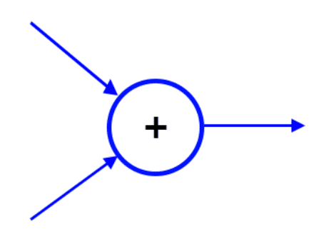
Add layer with two inputs
Since this cannot be represented as a linear stack of layers due to the multiple inputs, we would be unable to define it using a Sequential object. Here’s where Keras’ functional interface comes in. We can define an Add layer with two input tensors as such:
from tensorflow.keras.layers import Add
add_layer = Add()([layer1, layer2])
Now that we’ve seen a quick example of the functional interface, let’s take a look at what the LeNet5 model that we defined by instantiating a Sequential class would look like using a functional interface.
import tensorflow as tf
from tensorflow.keras.layers import Dense, Input, Flatten, Conv2D, MaxPool2D
from tensorflow.keras.models import Model

input_layer = Input(shape=(32,32,3,))
x = Conv2D(filters=6, kernel_size=(5,5), padding="same", activation="relu")(input_layer)
x = MaxPool2D(pool_size=(2,2))(x)
x = Conv2D(filters=16, kernel_size=(5,5), padding="same", activation="relu")(x)
x = MaxPool2D(pool_size=(2, 2))(x)
x = Conv2D(filters=120, kernel_size=(5,5), padding="same", activation="relu")(x)
x = Flatten()(x)
x = Dense(units=84, activation="relu")(x)
x = Dense(units=10, activation="softmax")(x)

model = Model(inputs=input_layer, outputs=x)

print(model.summary())
And looking at the model summary,
_________________________________________________________________
 Layer (type)                Output Shape              Param #
=================================================================
 input_2 (InputLayer)        [(None, 32, 32, 3)]       0

 conv2d_6 (Conv2D)           (None, 32, 32, 6)         456

 max_pooling2d_2 (MaxPooling  (None, 16, 16, 6)        0
 2D)

 conv2d_7 (Conv2D)           (None, 16, 16, 16)        2416

 max_pooling2d_3 (MaxPooling  (None, 8, 8, 16)         0
 2D)

 conv2d_8 (Conv2D)           (None, 8, 8, 120)         48120

 flatten_2 (Flatten)         (None, 7680)              0

 dense_4 (Dense)             (None, 84)                645204

 dense_5 (Dense)             (None, 10)                850

=================================================================
Total params: 697,046
Trainable params: 697,046
Non-trainable params: 0
_________________________________________________________________
As we can see, the model architecture is the same for both LeNet5 models that we have implemented using the functional interface or the Sequential class.
Now that we’ve seen how to use Keras’ functional interface, let’s look at a model architecture that we can implement using the functional interface but not with the Sequential class. For this example, we’ll look at the residual block introduced in ResNet. Visually, the residual block looks like this:
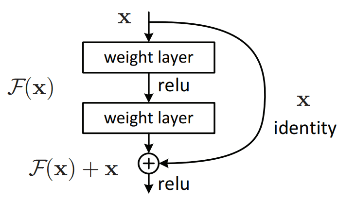
Residual block, source: https://arxiv.org/pdf/1512.03385.pdf
We can see that a model defined using the Sequential class would be unable to construct such a block due to the skip connection which prevents this block from being represented as a simple stack of layers. Using the functional interface, this is one way we can define a ResNet block:
def residual_block(x, filters):
  # store the input tensor to be added later as the identity
  identity = x
  # change the strides to do like pooling layer (need to see whether we connect before or after this layer though)
  x = Conv2D(filters = filters, kernel_size=(3, 3), strides = (1, 1), padding="same")(x)
  x = BatchNormalization()(x)
  x = relu(x)
  x = Conv2D(filters = filters, kernel_size=(3, 3), padding="same")(x)
  x = BatchNormalization()(x)
  x = Add()([identity, x])
  x = relu(x)

  return x
Then, we can build a simple network using these residual blocks using the functional interface as well.
input_layer = Input(shape=(32,32,3,))
x = Conv2D(filters=32, kernel_size=(3, 3), padding="same", activation="relu")(input_layer)
x = residual_block(x, 32)
x = Conv2D(filters=64, kernel_size=(3, 3), strides=(2, 2), padding="same", activation="relu")(x)
x = residual_block(x, 64)
x = Conv2D(filters=128, kernel_size=(3, 3), strides=(2, 2), padding="same", activation="relu")(x)
x = residual_block(x, 128)
x = Flatten()(x)
x = Dense(units=84, activation="relu")(x)
x = Dense(units=10, activation="softmax")(x)

model = Model(inputs=input_layer, outputs = x)
print(model.summary())

model.compile(optimizer="adam", loss=tf.keras.losses.SparseCategoricalCrossentropy(), metrics="acc")

history = model.fit(x=trainX, y=trainY, batch_size=256, epochs=10, validation_data=(testX, testY))
Running this code and looking at the model summary and training results,
__________________________________________________________________________________________________
 Layer (type)                   Output Shape         Param #     Connected to
==================================================================================================
 input_1 (InputLayer)           [(None, 32, 32, 3)]  0           []

 conv2d (Conv2D)                (None, 32, 32, 32)   896         ['input_1[0][0]']

 conv2d_1 (Conv2D)              (None, 32, 32, 32)   9248        ['conv2d[0][0]']

 batch_normalization (BatchNorm  (None, 32, 32, 32)  128         ['conv2d_1[0][0]']
 alization)

 tf.nn.relu (TFOpLambda)        (None, 32, 32, 32)   0
['batch_normalization[0][0]']

 conv2d_2 (Conv2D)              (None, 32, 32, 32)   9248        ['tf.nn.relu[0][0]']

 batch_normalization_1 (BatchNo  (None, 32, 32, 32)  128         ['conv2d_2[0][0]']
 rmalization)

 add (Add)                      (None, 32, 32, 32)   0           ['conv2d[0][0]',
                                                                  'batch_normalization_1[0][0]']

 tf.nn.relu_1 (TFOpLambda)      (None, 32, 32, 32)   0           ['add[0][0]']

 conv2d_3 (Conv2D)              (None, 16, 16, 64)   18496       ['tf.nn.relu_1[0][0]']

 conv2d_4 (Conv2D)              (None, 16, 16, 64)   36928       ['conv2d_3[0][0]']

 batch_normalization_2 (BatchNo  (None, 16, 16, 64)  256         ['conv2d_4[0][0]']
 rmalization)

 tf.nn.relu_2 (TFOpLambda)      (None, 16, 16, 64)   0
['batch_normalization_2[0][0]']

 conv2d_5 (Conv2D)              (None, 16, 16, 64)   36928       ['tf.nn.relu_2[0][0]']

 batch_normalization_3 (BatchNo  (None, 16, 16, 64)  256         ['conv2d_5[0][0]']
 rmalization)

 add_1 (Add)                    (None, 16, 16, 64)   0           ['conv2d_3[0][0]',
                                                                  'batch_normalization_3[0][0]']

 tf.nn.relu_3 (TFOpLambda)      (None, 16, 16, 64)   0           ['add_1[0][0]']

 conv2d_6 (Conv2D)              (None, 8, 8, 128)    73856       ['tf.nn.relu_3[0][0]']

 conv2d_7 (Conv2D)              (None, 8, 8, 128)    147584      ['conv2d_6[0][0]']

 batch_normalization_4 (BatchNo  (None, 8, 8, 128)   512         ['conv2d_7[0][0]']
 rmalization)

 tf.nn.relu_4 (TFOpLambda)      (None, 8, 8, 128)    0
['batch_normalization_4[0][0]']

 conv2d_8 (Conv2D)              (None, 8, 8, 128)    147584      ['tf.nn.relu_4[0][0]']

 batch_normalization_5 (BatchNo  (None, 8, 8, 128)   512         ['conv2d_8[0][0]']
 rmalization)

 add_2 (Add)                    (None, 8, 8, 128)    0           ['conv2d_6[0][0]',
                                                                  'batch_normalization_5[0][0]']

 tf.nn.relu_5 (TFOpLambda)      (None, 8, 8, 128)    0           ['add_2[0][0]']

 flatten (Flatten)              (None, 8192)         0           ['tf.nn.relu_5[0][0]']

 dense (Dense)                  (None, 84)           688212      ['flatten[0][0]']

 dense_1 (Dense)                (None, 10)           850         ['dense[0][0]']

==================================================================================================
Total params: 1,171,622
Trainable params: 1,170,726
Non-trainable params: 896
__________________________________________________________________________________________________
None
Epoch 1/10
196/196 [==============================] - 21s 46ms/step - loss: 3.4463
acc: 0.3635 - val_loss: 1.8015 - val_acc: 0.3459
Epoch 2/10
196/196 [==============================] - 8s 43ms/step - loss: 1.3267 - acc: 0.5200 - val_loss: 1.3895 - val_acc: 0.5069
Epoch 3/10
196/196 [==============================] - 8s 43ms/step - loss: 1.1095 - acc: 0.6062 - val_loss: 1.2008 - val_acc: 0.5651
Epoch 4/10
196/196 [==============================] - 9s 44ms/step - loss: 0.9618 - acc: 0.6585 - val_loss: 1.5411 - val_acc: 0.5226
Epoch 5/10
196/196 [==============================] - 9s 44ms/step - loss: 0.8656 - acc: 0.6968 - val_loss: 1.1012 - val_acc: 0.6234
Epoch 6/10
196/196 [==============================] - 8s 43ms/step - loss: 0.7622 - acc: 0.7361 - val_loss: 1.1355 - val_acc: 0.6168
Epoch 7/10
196/196 [==============================] - 9s 44ms/step - loss: 0.6801 - acc: 0.7602 - val_loss: 1.1561 - val_acc: 0.6187
Epoch 8/10
196/196 [==============================] - 8s 43ms/step - loss: 0.6106 - acc: 0.7905 - val_loss: 1.1100 - val_acc: 0.6401
Epoch 9/10
196/196 [==============================] - 9s 43ms/step - loss: 0.5367 - acc: 0.8146 - val_loss: 1.2989 - val_acc: 0.6058
Epoch 10/10
196/196 [==============================] - 9s 47ms/step - loss: 0.4776 - acc: 0.8348 - val_loss: 1.0098 - val_acc: 0.6757
And combining the code for our simple network using residual blocks,
import tensorflow as tf
from tensorflow import keras
from keras.layers import Input, Conv2D, BatchNormalization, Add, MaxPool2D, Flatten, Dense
from keras.activations import relu
from tensorflow.keras.models import Model

def residual_block(x, filters):
  # store the input tensor to be added later as the identity
  identity = x
  # change the strides to do like pooling layer (need to see whether we connect before or after this layer though)
  x = Conv2D(filters = filters, kernel_size=(3, 3), strides = (1, 1), padding="same")(x)
  x = BatchNormalization()(x)
  x = relu(x)
  x = Conv2D(filters = filters, kernel_size=(3, 3), padding="same")(x)
  x = BatchNormalization()(x)
  x = Add()([identity, x])
  x = relu(x)

  return x

(trainX, trainY), (testX, testY) = keras.datasets.cifar10.load_data()

input_layer = Input(shape=(32,32,3,))
x = Conv2D(filters=32, kernel_size=(3, 3), padding="same", activation="relu")(input_layer)
x = residual_block(x, 32)
x = Conv2D(filters=64, kernel_size=(3, 3), strides=(2, 2), padding="same", activation="relu")(x)
x = residual_block(x, 64)
x = Conv2D(filters=128, kernel_size=(3, 3), strides=(2, 2), padding="same", activation="relu")(x)
x = residual_block(x, 128)
x = Flatten()(x)
x = Dense(units=84, activation="relu")(x)
x = Dense(units=10, activation="softmax")(x)

model = Model(inputs=input_layer, outputs = x)
print(model.summary())

model.compile(optimizer="adam", loss=tf.keras.losses.SparseCategoricalCrossentropy(), metrics="acc")

history = model.fit(x=trainX, y=trainY, batch_size=256, epochs=10, validation_data=(testX, testY))
Subclassing keras.Model
Keras also provides an object-oriented approach to creating models, which would help with reusability and allows us to represent the models that we want to create as classes. This representation might be more intuitive, since we can think about models as a set of layers strung together to form our network.
To begin subclassing keras.Model, we first need to import it.
from tensorflow.keras.models import Model
Then, we can start subclassing Model. First, we need to build the layers that we want to use in our method calls since we only want to instantiate these layers once instead of each time we call our model. To keep in line with previous examples, let’s build a LeNet5 model here as well.
class LeNet5(tf.keras.Model):
  def __init__(self):
    super(LeNet5, self).__init__()
    #creating layers in initializer
    self.conv1 = Conv2D(filters=6, kernel_size=(5,5), padding="same", activation="relu")
    self.max_pool2x2 = MaxPool2D(pool_size=(2,2))
    self.conv2 = Conv2D(filters=16, kernel_size=(5,5), padding="same", activation="relu")
    self.conv3 = Conv2D(filters=120, kernel_size=(5,5), padding="same", activation="relu")
    self.flatten = Flatten()
    self.fc2 = Dense(units=84, activation="relu")
    self.fc3 = Dense(units=10, activation="softmax")
Then, we override the call method to define what happens when the model is called. We override it with our model which uses the layers that we have built in the initializer.
def call(self, input_tensor):
  # don't create layers here, need to create the layers in initializer,
  # otherwise you will get the tf.Variable can only be created once error
  conv1 = self.conv1(input_tensor)
  maxpool1 = self.max_pool2x2(conv1)
  conv2 = self.conv2(maxpool1)
  maxpool2 = self.max_pool2x2(conv2)
  conv3 = self.conv3(maxpool2)
  flatten = self.flatten(conv3)
  fc2 = self.fc2(flatten)
  fc3 = self.fc3(fc2)

  return fc3
It is important to have all the layers created at the class constructor, not inside the call() method. It is because the call() method will be invoked multiple times with different input tensor. But we want to use the same layer objects in each call so we can optimize their weight. We can then instantiate our new LeNet5 class and use it as part of a model:
input_layer = Input(shape=(32,32,3,))
x = LeNet5()(input_layer)

model = Model(inputs=input_layer, outputs=x)

print(model.summary(expand_nested=True))
And we can see that the model has the same number of parameters as the previous two versions of LeNet5 that we built previously and has the same structure within it as well.
_________________________________________________________________
 Layer (type)                Output Shape              Param #
=================================================================
 input_1 (InputLayer)        [(None, 32, 32, 3)]       0

 le_net5 (LeNet5)            (None, 10)                697046
|¯¯¯¯¯¯¯¯¯¯¯¯¯¯¯¯¯¯¯¯¯¯¯¯¯¯¯¯¯¯¯¯¯¯¯¯¯¯¯¯¯¯¯¯¯¯¯¯¯¯¯¯¯¯¯¯¯¯¯¯¯¯¯|
| conv2d (Conv2D)           multiple                  456       |
|                                                               |
| max_pooling2d (MaxPooling2D  multiple               0         |
| )                                                             |
|                                                               |
| conv2d_1 (Conv2D)         multiple                  2416      |
|                                                               |
| conv2d_2 (Conv2D)         multiple                  48120     |
|                                                               |
| flatten (Flatten)         multiple                  0         |
|                                                               |
| dense (Dense)             multiple                  645204    |
|                                                               |
| dense_1 (Dense)           multiple                  850       |
¯¯¯¯¯¯¯¯¯¯¯¯¯¯¯¯¯¯¯¯¯¯¯¯¯¯¯¯¯¯¯¯¯¯¯¯¯¯¯¯¯¯¯¯¯¯¯¯¯¯¯¯¯¯¯¯¯¯¯¯¯¯¯¯¯
=================================================================
Total params: 697,046
Trainable params: 697,046
Non-trainable params: 0
_________________________________________________________________
Combining all of the code to create our LeNet5 subclass of keras.Model,
import tensorflow as tf
from tensorflow.keras.layers import Dense, Input, Flatten, Conv2D, MaxPool2D
from tensorflow.keras.models import Model

class LeNet5(tf.keras.Model):
  def __init__(self):
    super(LeNet5, self).__init__()
    #creating layers in initializer
    self.conv1 = Conv2D(filters=6, kernel_size=(5,5), padding="same", activation="relu")
    self.max_pool2x2 = MaxPool2D(pool_size=(2,2))
    self.conv2 = Conv2D(filters=16, kernel_size=(5,5), padding="same", activation="relu")
    self.conv3 = Conv2D(filters=120, kernel_size=(5,5), padding="same", activation="relu")
    self.flatten = Flatten()
    self.fc2 = Dense(units=84, activation="relu")
    self.fc3=Dense(units=10, activation="softmax")

  def call(self, input_tensor):
    #don't add layers here, need to create the layers in initializer, otherwise you will get the tf.Variable can only be created once error
    x = self.conv1(input_tensor)
    x = self.max_pool2x2(x)
    x = self.conv2(x)
    x = self.max_pool2x2(x)
    x = self.conv3(x)
    x = self.flatten(x)
    x = self.fc2(x)
    x = self.fc3(x)
    return x
input_layer = Input(shape=(32,32,3,))
x = LeNet5()(input_layer)
model = Model(inputs=input_layer, outputs=x)
print(model.summary(expand_nested=True))
Further Reading
This section provides more resources on the topic if you are looking to go deeper.
Papers:
- Deep Residual Learning for Image Recognition (the ResNet paper)
APIs:
Summary
In this post, you have seen three different ways to create models in Keras, in particular, using the Sequential class, functional interface and subclassing keras.Model. You have also seen examples of the same LeNet5 model being built using the different methods and seen a use case which can be done using the functional interface but not with the Sequential class.
Specifically, you learned:
- Different ways that Keras offers to build models
- How to use the Sequential class, functional interface, and subclassing keras.Model to build Keras models
- When to use the different methods to create Keras models
The post Three Ways to Build Machine Learning Models in Keras appeared first on Machine Learning Mastery.